Chapter 10. Classification Models for Business Decisions

Classification is one of the most widely applied machine learning techniques in business analytics. From predicting customer churn and detecting fraudulent transactions to assessing credit risk and targeting marketing campaigns, classification models help organizations make data-driven decisions that directly impact revenue, risk, and customer satisfaction.

This chapter introduces the fundamental concepts of classification, explores both basic and advanced algorithms, addresses the critical challenge of class imbalance, and demonstrates how to interpret and evaluate classification models. We conclude with a comprehensive Python implementation focused on credit scoring—a classic business application where accurate classification can mean the difference between profit and loss.

10.1 Classification Problems in Business

Classification is a supervised learning task where the goal is to predict a categorical label (the target  or class ) based on input features. Unlike regression, which predicts continuous values, classification assigns observations to discrete categories.

Common Business Classification Problems

Customer Churn Prediction
 Identifying customers likely to stop using a service or product. Telecom companies, subscription services, and banks use churn models to proactively retain valuable customers through targeted interventions.

• Target:  Churned (1) vs. Retained (0)
• Features:  Usage patterns, customer demographics, service complaints, contract type
• Business Impact:  Reducing churn by even 5% can significantly increase lifetime customer value

Fraud Detection
 Detecting fraudulent transactions in credit cards, insurance claims, or online payments.   Recent research  shows that combining traditional ML models with techniques like SMOTE can achieve over 99% accuracy in fraud detection.

• Target:  Fraudulent (1) vs. Legitimate (0)
• Features:  Transaction amount, location, time, merchant category, user behavior
• Business Impact:  Prevents financial losses while minimizing false positives that frustrate customers

Credit Scoring
 Assessing the creditworthiness of loan applicants to determine approval and interest rates. Financial institutions rely on classification models to balance risk and opportunity.

• Target:  Default (1) vs. Repay (0)
• Features:  Income, employment history, existing debt, credit history, loan amount
• Business Impact:  Reduces default rates while expanding access to credit for qualified borrowers

Marketing Response Prediction
 Predicting which customers will respond to marketing campaigns, enabling targeted outreach and efficient resource allocation.

• Target:  Responder (1) vs. Non-responder (0)
• Features:  Past purchase behavior, demographics, engagement metrics
• Business Impact:  Increases campaign ROI and reduces marketing costs

Medical Diagnosis
 Classifying patients as having or not having a particular condition based on symptoms, test results, and medical history.

• Target:  Disease Present (1) vs. Absent (0)
• Features:  Lab results, vital signs, patient history, imaging data
• Business Impact:  Improves patient outcomes and optimizes healthcare resource allocation

Key Characteristics of Business Classification Problems

1. Imbalanced Classes:  In most business scenarios, the event of interest (fraud, churn, default) is rare, creating significant class imbalance
2. Cost-Sensitive:  Misclassification costs are often asymmetric—missing a fraud case may be more costly than a false alarm
3. Interpretability Matters:  Stakeholders often need to understand why  a prediction was made, especially in regulated industries
4. Dynamic Patterns:  Customer behavior and fraud tactics evolve, requiring models to be regularly updated

10.2 Basic Algorithms

10.2.1 Logistic Regression

Despite its name, logistic regression is a classification  algorithm. It models the probability that an observation belongs to a particular class using the logistic (sigmoid) function.

Mathematical Foundation

For binary classification, logistic regression models:

P(y=1∣X)=1+e−(β0​+β1​x1​+β2​x2​+...+βp​xp​)​

Where:

• P(y=1∣X) is the probability of the positive class
• β0​,β1​,...,βp​ are coefficients learned from data
• The decision boundary is typically set at P=0.5

Advantages

• Interpretable:  Coefficients indicate feature importance and direction of effect
• Probabilistic output:  Provides calibrated probability estimates
• Efficient:  Fast to train and predict, even on large datasets
• Regularization:  L1 (Lasso) and L2 (Ridge) regularization prevent overfitting

Limitations

• Linear decision boundary:  Assumes a linear relationship between features and log-odds
• Feature engineering required:  May need polynomial features or interactions for complex patterns
• Sensitive to outliers:  Extreme values can influence coefficients

Business Use Cases

• Credit scoring (interpretability required for regulatory compliance)
• Email spam detection
• Customer conversion prediction

AI Prompt for Logistic Regression:

"Explain how logistic regression coefficients can be interpreted in a credit scoring model.
If the coefficient for 'income' is 0.05, what does this mean for loan approval probability?"

10.2.2 Decision Trees

Decision trees recursively partition the feature space into regions, making predictions based on simple decision rules learned from data. Each internal node represents a test on a feature, each branch represents an outcome, and each leaf node represents a class label.

How Decision Trees Work

1. Splitting:  At each node, the algorithm selects the feature and threshold that best separates the classes (using metrics like Gini impurity or information gain)
2. Recursion:  The process repeats for each child node until a stopping criterion is met (max depth, minimum samples, purity)
3. Prediction:  New observations traverse the tree from root to leaf, following the decision rules

Key Hyperparameters

• max_depth : Maximum depth of the tree (controls complexity)
• min_samples_split : Minimum samples required to split a node
• min_samples_leaf : Minimum samples required in a leaf node
• criterion : Splitting criterion ('gini' or 'entropy')

Advantages

• Highly interpretable:  Can be visualized and explained to non-technical stakeholders
• Non-linear:  Captures complex, non-linear relationships
• No feature scaling needed:  Works with features on different scales
• Handles mixed data types:  Works with both numerical and categorical features

Limitations

• Overfitting:  Deep trees can memorize training data
• Instability:  Small changes in data can lead to very different trees
• Biased toward dominant classes:  In imbalanced datasets, may favor the majority class

Business Use Cases

• Customer segmentation
• Loan approval decisions (when interpretability is critical)
• Medical diagnosis

AI Prompt for Decision Trees:

"I have a decision tree for churn prediction with 15 leaf nodes. How can I simplify this tree
to make it more interpretable for business stakeholders while maintaining reasonable accuracy?"

10.3 More Advanced Algorithms

10.3.1 Random Forests  

Random Forest is an ensemble method  that combines multiple decision trees to improve prediction accuracy and reduce overfitting. Each tree is trained on a random subset of data (bootstrap sample) and considers only a random subset of features at each split.

Key Concepts:

• Bagging (Bootstrap Aggregating):  Each tree sees a different sample of data
• Feature Randomness:  Each split considers only a subset of features
• Voting:  Final prediction is the majority vote (classification) or average (regression)

Advantages:

• Robust:  Less prone to overfitting than single decision trees
• Feature importance:  Provides measures of feature relevance
• Handles high-dimensional data:  Works well even with many features
• Minimal hyperparameter tuning:  Often performs well with default settings

Recent studies  show Random Forest achieving 99.5% accuracy in credit card fraud detection when combined with SMOTE for handling class imbalance.

10.3.2 Gradient Boosting

Gradient Boosting builds trees sequentially , where each new tree corrects the errors of the previous ensemble. Popular implementations include XGBoost, LightGBM, and CatBoost. They are one of the best models. For rich categorical data we recommend CatBoost.

Key Concepts:

• Sequential learning:  Trees are added one at a time
• Error correction:  Each tree focuses on the residuals (errors) of the previous ensemble
• Learning rate:  Controls how much each tree contributes to the final prediction

Advantages:

• State-of-the-art performance:  Often wins machine learning competitions
• Handles complex patterns:  Captures intricate relationships in data
• Built-in regularization:  Techniques like shrinkage prevent overfitting

Disadvantages:

• Computationally expensive:  Slower to train than Random Forest
• More hyperparameters:  Requires careful tuning
• Less interpretable:  Harder to explain than single trees

Business Applications:

• Credit scoring (highest accuracy)
• Fraud detection
• Customer lifetime value prediction

10.3.3 Neural Networks

Neural networks, particularly deep learning  models, have gained prominence in classification tasks involving unstructured data (images, text, audio). For structured business data, simpler models often suffice, but neural networks can capture highly complex patterns.

Basic Architecture:

• Input layer:  One neuron per feature
• Hidden layers:  Intermediate layers that learn representations
• Output layer:  Neurons corresponding to classes (with softmax activation for multi-class)

Advantages:

• Universal approximators:  Can model any function given enough neurons
• Automatic feature learning:  Learns relevant features from raw data
• Scalability:  Handles massive datasets efficiently with GPUs

Disadvantages:

• Black box:  Difficult to interpret
• Data hungry:  Requires large amounts of training data
• Computationally intensive:  Needs significant resources
• Hyperparameter sensitivity:  Many parameters to tune

Business Use Cases:

• Image-based fraud detection (e.g., check fraud)
• Natural language processing for customer sentiment
• Complex pattern recognition in high-dimensional data

Example  ANN - ppp

10.4 Handling Class Imbalance

Class imbalance occurs when one class significantly outnumbers the other(s). In business problems like fraud detection (0.17% fraud rate) or churn prediction (typically 5-20% churn), this is the norm rather than the exception.

Why Class Imbalance is Problematic

1. Biased Models:  Algorithms optimize for overall accuracy, which can be achieved by simply predicting the majority class
2. Poor Minority Class Performance:  The model fails to learn patterns in the rare but important class
3. Misleading Metrics:  99% accuracy is meaningless if it's achieved by predicting "no fraud" for every transaction

Techniques for Handling Class Imbalance

1. Resampling Methods

Undersampling:  Reduce the number of majority class samples

• Random Undersampling:  Randomly remove majority class samples
• Tomek Links:  Remove majority class samples that are close to minority class samples
• Pros:  Faster training, balanced dataset
• Cons:  Loss of potentially useful information

Oversampling:  Increase the number of minority class samples

• Random Oversampling:  Duplicate minority class samples
• Pros:  No information loss
• Cons:  Risk of overfitting, increased training time

SMOTE (Synthetic Minority Over-sampling Technique)

SMOTE creates synthetic  minority class samples by interpolating between existing minority class samples.   Research shows  that SMOTE significantly improves model performance on imbalanced datasets.

How SMOTE Works:

1. For each minority class sample, find its k nearest neighbors (typically k=5)
2. Randomly select one of these neighbors
3. Create a synthetic sample along the line segment connecting the two samples

from imblearn.over_sampling import SMOTE

smote = SMOTE(random_state=42)

X_resampled, y_resampled = smote.fit_resample(X_train, y_train)

SMOTE-Tomek:  Combines SMOTE oversampling with Tomek Links undersampling to clean the decision boundary

2. Algorithm-Level Techniques

Class Weights:  Assign higher penalties to misclassifying the minority class

from sklearn.linear_model import LogisticRegression

model = LogisticRegression(class_weight='balanced')  

Threshold Adjustment:  Instead of using 0.5 as the decision threshold, optimize it based on business costs

3. Ensemble Methods

Balanced Random Forest:  Each tree is trained on a balanced bootstrap sample

from imblearn.ensemble import BalancedRandomForestClassifier

model = BalancedRandomForestClassifier(random_state=42)

EasyEnsemble:  Creates multiple balanced subsets and trains an ensemble

Choosing the Right Technique

• Small datasets:  SMOTE or SMOTE-Tomek
• Large datasets:  Undersampling or class weights
• Extreme imbalance (< 1% minority):  Combination of techniques
• Real-time systems:  Class weights (no preprocessing needed)

10.5 Interpreting Classification Models

10.5.1 Coefficients, Feature Importance, and Partial Dependence (Conceptual)

Logistic Regression Coefficients

Coefficients indicate the change in log-odds for a one-unit increase in the feature:

• Positive coefficient:  Increases probability of positive class
• Negative coefficient:  Decreases probability of positive class
• Magnitude:  Indicates strength of effect

Example:  In credit scoring, if the coefficient for income  is 0.0005, then a $10,000 increase in income increases the log-odds of approval by 5.

Feature Importance (Tree-Based Models)

Feature importance measures how much each feature contributes to reducing impurity across all trees:

• Higher values:  More important features
• Interpretation:  Relative, not absolute

import pandas as pd

importances = model.feature_importances_

feature_importance_df = pd.DataFrame({

    'feature': X_train.columns,

    'importance': importances

}).sort_values('importance', ascending=False)

Partial Dependence Plots (PDP)

PDPs show the marginal effect of a feature on the predicted outcome, holding other features constant. They help visualize non-linear relationships.

SHAP (SHapley Additive exPlanations)

SHAP values provide a unified measure of feature importance based on game theory, showing how much each feature contributes to a specific prediction.

10.5.2 Metrics: Precision, Recall, Confusion Matrix, F1, AUC

Accuracy alone is insufficient for evaluating classification models, especially with imbalanced data. We need a comprehensive set of metrics.

Confusion Matrix

A confusion matrix summarizes prediction results:

Key Metrics

Accuracy:  Overall correctness

Accuracy=TP+TN+FP+FNTP+TN​

• Limitation:  Misleading with imbalanced data

Precision:  Of all positive predictions, how many were correct?

Precision=TP+FPTP​

• Business Interpretation:  In fraud detection, high precision means few false alarms

Recall (Sensitivity):  Of all actual positives, how many did we catch?

Recall=TP+FNTP​

• Business Interpretation:  In fraud detection, high recall means we catch most fraud cases

F1-Score:  Harmonic mean of precision and recall

F1 = 2×Precision+RecallPrecision×Recall​

• Use Case:  When you need a balance between precision and recall

Specificity:  Of all actual negatives, how many did we correctly identify?

Specificity=TN+FPTN​

ROC Curve and AUC

The Receiver Operating Characteristic (ROC)  curve plots True Positive Rate (Recall) vs. False Positive Rate at various threshold settings.

AUC (Area Under the Curve):  Measures the model's ability to distinguish between classes

• AUC = 1.0:  Perfect classifier
• AUC = 0.5:  Random guessing
• AUC > 0.8:  Generally considered good

Business Interpretation:  AUC represents the probability that the model ranks a random positive example higher than a random negative example.

Choosing the Right Metric

• Fraud detection:  Prioritize Recall  (catch all fraud) and AUC
• Spam filtering:  Prioritize Precision  (avoid false positives)
• Credit scoring:  Balance Precision  and Recall  (F1-Score), consider business costs
• Medical diagnosis:  Prioritize Recall  (don't miss diseases)

10.6 Implementing Classification in Python

Credit Scoring Example: Complete Implementation

We'll build a comprehensive credit scoring model using a synthetic dataset that mimics real-world credit data. This example demonstrates data preparation, handling class imbalance, model training, evaluation, and interpretation.

# Import necessary libraries

import numpy as np

import pandas as pd

import matplotlib.pyplot as plt

import seaborn as sns

from sklearn.model_selection import train_test_split, cross_val_score, GridSearchCV

from sklearn.preprocessing import StandardScaler

from sklearn.linear_model import LogisticRegression

from sklearn.tree import DecisionTreeClassifier, plot_tree

from sklearn.ensemble import RandomForestClassifier, GradientBoostingClassifier

from sklearn.metrics import (classification_report, confusion_matrix,

                             roc_curve, roc_auc_score, precision_recall_curve,

                             f1_score, accuracy_score)

from imblearn.over_sampling import SMOTE

from imblearn.combine import SMOTETomek

import warnings

warnings.filterwarnings('ignore')

# Set style for better visualizations

sns.set_style('whitegrid')

plt.rcParams['figure.figsize'] = (12, 6)

print("Libraries imported successfully!")

Step 1: Generate Synthetic Credit Scoring Dataset

# Set random seed for reproducibility

np.random.seed(42)

# Generate synthetic credit data

n_samples = 10000

# Create features

data = {

    'age': np.random.randint(18, 70, n_samples),

    'income': np.random.gamma(shape=2, scale=25000, size=n_samples),  # Right-skewed income

    'credit_history_length': np.random.randint(0, 30, n_samples),  # Years

    'num_credit_lines': np.random.poisson(lam=3, size=n_samples),

    'debt_to_income_ratio': np.random.beta(a=2, b=5, size=n_samples),  # Typically < 0.5

    'num_late_payments': np.random.poisson(lam=1, size=n_samples),

    'credit_utilization': np.random.beta(a=2, b=3, size=n_samples),  # 0 to 1

    'num_inquiries_6m': np.random.poisson(lam=1, size=n_samples),

    'loan_amount': np.random.gamma(shape=2, scale=10000, size=n_samples),

    'employment_length': np.random.randint(0, 25, n_samples),

}

df = pd.DataFrame(data)

# Create target variable (default) based on realistic risk factors

# Higher risk of default with: low income, high debt ratio, late payments, high utilization

risk_score = (

    -0.00001 * df['income'] +

    0.5 * df['debt_to_income_ratio'] +

    0.3 * df['num_late_payments'] +

    0.4 * df['credit_utilization'] +

    0.1 * df['num_inquiries_6m'] +

    -0.02 * df['credit_history_length'] +

    -0.01 * df['employment_length'] +

    np.random.normal(0, 0.3, n_samples)  # Add noise

)

# Convert risk score to probability and then to binary outcome

default_probability = 1 / (1 + np.exp(-risk_score))

df['default'] = (default_probability > 0.7).astype(int)  # Create imbalance

# Add some categorical features

df['home_ownership'] = np.random.choice(['RENT', 'OWN', 'MORTGAGE'], n_samples, p=[0.3, 0.2, 0.5])

df['loan_purpose'] = np.random.choice(['debt_consolidation', 'credit_card', 'home_improvement',

                                       'major_purchase', 'other'], n_samples)

print(f"Dataset shape: {df.shape}")

print(f"\nFirst few rows:")

print(df.head())

print(f"\nClass distribution:")

print(df['default'].value_counts())

print(f"\nDefault rate: {df['default'].mean():.2%}")

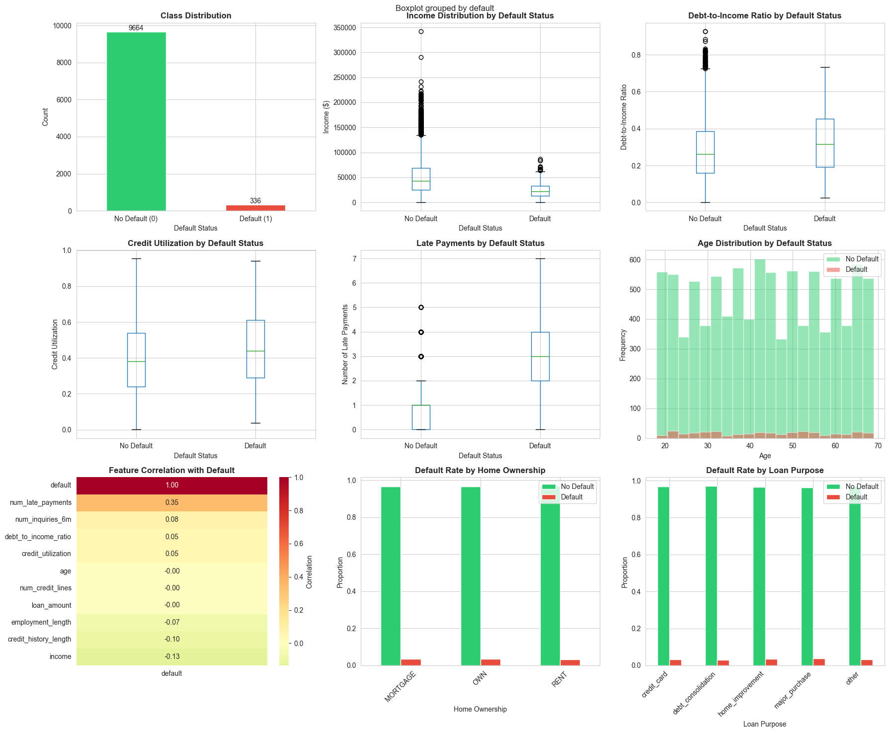
Step 2: Exploratory Data Analysis (EDA)

# Create comprehensive EDA visualizations

fig, axes = plt.subplots(3, 3, figsize=(18, 15))

fig.suptitle('Credit Scoring Dataset: Exploratory Data Analysis', fontsize=16, fontweight='bold')

# 1. Class distribution

ax = axes[0, 0]

df['default'].value_counts().plot(kind='bar', ax=ax, color=['#2ecc71', '#e74c3c'])

ax.set_title('Class Distribution', fontweight='bold')

ax.set_xlabel('Default Status')

ax.set_ylabel('Count')

ax.set_xticklabels(['No Default (0)', 'Default (1)'], rotation=0)

for container in ax.containers:

    ax.bar_label(container)

# 2. Income distribution by default status

ax = axes[0, 1]

df.boxplot(column='income', by='default', ax=ax)

ax.set_title('Income Distribution by Default Status', fontweight='bold')

ax.set_xlabel('Default Status')

ax.set_ylabel('Income ($)')

plt.sca(ax)

plt.xticks([1, 2], ['No Default', 'Default'])

# 3. Debt-to-Income Ratio by default status

ax = axes[0, 2]

df.boxplot(column='debt_to_income_ratio', by='default', ax=ax)

ax.set_title('Debt-to-Income Ratio by Default Status', fontweight='bold')

ax.set_xlabel('Default Status')

ax.set_ylabel('Debt-to-Income Ratio')

plt.sca(ax)

plt.xticks([1, 2], ['No Default', 'Default'])

# 4. Credit utilization by default status

ax = axes[1, 0]

df.boxplot(column='credit_utilization', by='default', ax=ax)

ax.set_title('Credit Utilization by Default Status', fontweight='bold')

ax.set_xlabel('Default Status')

ax.set_ylabel('Credit Utilization')

plt.sca(ax)

plt.xticks([1, 2], ['No Default', 'Default'])

# 5. Number of late payments

ax = axes[1, 1]

df.boxplot(column='num_late_payments', by='default', ax=ax)

ax.set_title('Late Payments by Default Status', fontweight='bold')

ax.set_xlabel('Default Status')

ax.set_ylabel('Number of Late Payments')

plt.sca(ax)

plt.xticks([1, 2], ['No Default', 'Default'])

# 6. Age distribution

ax = axes[1, 2]

df[df['default']==0]['age'].hist(bins=20, alpha=0.5, label='No Default', ax=ax, color='#2ecc71')

df[df['default']==1]['age'].hist(bins=20, alpha=0.5, label='Default', ax=ax, color='#e74c3c')

ax.set_title('Age Distribution by Default Status', fontweight='bold')

ax.set_xlabel('Age')

ax.set_ylabel('Frequency')

ax.legend()

# 7. Correlation heatmap

ax = axes[2, 0]

numeric_cols = df.select_dtypes(include=[np.number]).columns

corr_matrix = df[numeric_cols].corr()

sns.heatmap(corr_matrix[['default']].sort_values(by='default', ascending=False),

            annot=True, fmt='.2f', cmap='RdYlGn_r', center=0, ax=ax, cbar_kws={'label': 'Correlation'})

ax.set_title('Feature Correlation with Default', fontweight='bold')

# 8. Home ownership distribution

ax = axes[2, 1]

pd.crosstab(df['home_ownership'], df['default'], normalize='index').plot(kind='bar', ax=ax,

                                                                          color=['#2ecc71', '#e74c3c'])

ax.set_title('Default Rate by Home Ownership', fontweight='bold')

ax.set_xlabel('Home Ownership')

ax.set_ylabel('Proportion')

ax.legend(['No Default', 'Default'])

ax.set_xticklabels(ax.get_xticklabels(), rotation=45)

# 9. Loan purpose distribution

ax = axes[2, 2]

pd.crosstab(df['loan_purpose'], df['default'], normalize='index').plot(kind='bar', ax=ax,

                                                                        color=['#2ecc71', '#e74c3c'])

ax.set_title('Default Rate by Loan Purpose', fontweight='bold')

ax.set_xlabel('Loan Purpose')

ax.set_ylabel('Proportion')

ax.legend(['No Default', 'Default'])

ax.set_xticklabels(ax.get_xticklabels(), rotation=45, ha='right')

plt.tight_layout()

plt.show()

# Print summary statistics

print("\n" + "="*60)

print("SUMMARY STATISTICS BY DEFAULT STATUS")

print("="*60)

print(df.groupby('default')[['income', 'debt_to_income_ratio', 'credit_utilization',

                              'num_late_payments', 'credit_history_length']].mean())

===========================================================

SUMMARY STATISTICS BY DEFAULT STATUS

============================================================

               income  debt_to_income_ratio  credit_utilization  \

default                                                          

0        51044.020129              0.283362            0.395485  

1        24959.954392              0.329210            0.449313  

         num_late_payments  credit_history_length  

default                                            

0                 0.918771              14.773282  

1                 2.833333               9.806548  

Step 3: Data Preprocessing

# Encode categorical variables

df_encoded = pd.get_dummies(df, columns=['home_ownership', 'loan_purpose'], drop_first=True)

# Separate features and target

X = df_encoded.drop('default', axis=1)

y = df_encoded['default']

# Split data

X_train, X_test, y_train, y_test = train_test_split(X, y, test_size=0.2, random_state=42, stratify=y)

print(f"Training set size: {X_train.shape}")

print(f"Test set size: {X_test.shape}")

print(f"\nTraining set class distribution:")

print(y_train.value_counts())

print(f"Default rate in training set: {y_train.mean():.2%}")

# Scale features

scaler = StandardScaler()

X_train_scaled = scaler.fit_transform(X_train)

X_test_scaled = scaler.transform(X_test)

# Convert back to DataFrame for easier handling

X_train_scaled = pd.DataFrame(X_train_scaled, columns=X_train.columns, index=X_train.index)

X_test_scaled = pd.DataFrame(X_test_scaled, columns=X_test.columns, index=X_test.index)

print("\nData preprocessing completed!")

Output

Training set size: (8000, 16)

Test set size: (2000, 16)

Training set class distribution:

default

0    7731

1     269

Name: count, dtype: int64

Default rate in training set: 3.36%

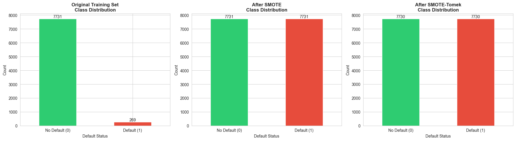
Step 4: Handle Class Imbalance with SMOTE

# Visualize class imbalance before and after SMOTE

fig, axes = plt.subplots(1, 3, figsize=(18, 5))

# Original distribution

ax = axes[0]

y_train.value_counts().plot(kind='bar', ax=ax, color=['#2ecc71', '#e74c3c'])

ax.set_title('Original Training Set\nClass Distribution', fontweight='bold', fontsize=12)

ax.set_xlabel('Default Status')

ax.set_ylabel('Count')

ax.set_xticklabels(['No Default (0)', 'Default (1)'], rotation=0)

for container in ax.containers:

    ax.bar_label(container)

# Apply SMOTE

smote = SMOTE(random_state=42)

X_train_smote, y_train_smote = smote.fit_resample(X_train_scaled, y_train)

# SMOTE distribution

ax = axes[1]

pd.Series(y_train_smote).value_counts().plot(kind='bar', ax=ax, color=['#2ecc71', '#e74c3c'])

ax.set_title('After SMOTE\nClass Distribution', fontweight='bold', fontsize=12)

ax.set_xlabel('Default Status')

ax.set_ylabel('Count')

ax.set_xticklabels(['No Default (0)', 'Default (1)'], rotation=0)

for container in ax.containers:

    ax.bar_label(container)

# Apply SMOTE-Tomek

smote_tomek = SMOTETomek(random_state=42)

X_train_smote_tomek, y_train_smote_tomek = smote_tomek.fit_resample(X_train_scaled, y_train)

# SMOTE-Tomek distribution

ax = axes[2]

pd.Series(y_train_smote_tomek).value_counts().plot(kind='bar', ax=ax, color=['#2ecc71', '#e74c3c'])

ax.set_title('After SMOTE-Tomek\nClass Distribution', fontweight='bold', fontsize=12)

ax.set_xlabel('Default Status')

ax.set_ylabel('Count')

ax.set_xticklabels(['No Default (0)', 'Default (1)'], rotation=0)

for container in ax.containers:

    ax.bar_label(container)

plt.tight_layout()

plt.show()

print(f"Original training set: {len(y_train)} samples")

print(f"After SMOTE: {len(y_train_smote)} samples")

print(f"After SMOTE-Tomek: {len(y_train_smote_tomek)} samples")

Output

Original training set: 8000 samples

After SMOTE: 15462 samples

After SMOTE-Tomek: 15460 samples

Step 5: Train Multiple Classification Models

# Define models

models = {

    'Logistic Regression': LogisticRegression(random_state=42, max_iter=1000),

    'Logistic Regression (Balanced)': LogisticRegression(random_state=42, max_iter=1000, class_weight='balanced'),

    'Decision Tree': DecisionTreeClassifier(random_state=42, max_depth=5),

    'Random Forest': RandomForestClassifier(random_state=42, n_estimators=100),

    'Gradient Boosting': GradientBoostingClassifier(random_state=42, n_estimators=100)

}

# Train models on original data

results_original = {}

for name, model in models.items():

    model.fit(X_train_scaled, y_train)

    y_pred = model.predict(X_test_scaled)

    y_pred_proba = model.predict_proba(X_test_scaled)[:, 1]

    results_original[name] = {

        'model': model,

        'y_pred': y_pred,

        'y_pred_proba': y_pred_proba,

        'accuracy': accuracy_score(y_test, y_pred),

        'f1': f1_score(y_test, y_pred),

        'auc': roc_auc_score(y_test, y_pred_proba)

    }

# Train models on SMOTE data

results_smote = {}

for name, model in models.items():

    if 'Balanced' in name:  # Skip balanced version for SMOTE

        continue

    model_smote = type(model)(**model.get_params())  # Create new instance

    model_smote.fit(X_train_smote, y_train_smote)

    y_pred = model_smote.predict(X_test_scaled)

    y_pred_proba = model_smote.predict_proba(X_test_scaled)[:, 1]

    results_smote[name + ' (SMOTE)'] = {

        'model': model_smote,

        'y_pred': y_pred,

        'y_pred_proba': y_pred_proba,

        'accuracy': accuracy_score(y_test, y_pred),

        'f1': f1_score(y_test, y_pred),

        'auc': roc_auc_score(y_test, y_pred_proba)

    }

# Combine results

all_results = {**results_original, **results_smote}

# Create comparison DataFrame

comparison_df = pd.DataFrame({

    name: {

        'Accuracy': results['accuracy'],

        'F1-Score': results['f1'],

        'AUC': results['auc']

    }

    for name, results in all_results.items()

}).T.sort_values('F1-Score', ascending=False)

print("\n" + "="*80)

print("MODEL PERFORMANCE COMPARISON")

print("="*80)

print(comparison_df.round(4))

Output:

================================================================================

MODEL PERFORMANCE COMPARISON

================================================================================

                                Accuracy  F1-Score     AUC

Logistic Regression               0.9785    0.6195  0.9712

Gradient Boosting                 0.9775    0.5872  0.9489

Gradient Boosting (SMOTE)         0.9605    0.5434  0.9575

Random Forest (SMOTE)             0.9680    0.5152  0.9488

Decision Tree                     0.9710    0.4630  0.8939

Logistic Regression (SMOTE)       0.9080    0.3987  0.9720

Random Forest                     0.9725    0.3956  0.9395

Logistic Regression (Balanced)    0.8970    0.3758  0.9717

Decision Tree (SMOTE)             0.9020    0.3423  0.8957

Step 6: Detailed Evaluation of Best Model

# Select best model (Random Forest with SMOTE)

best_model_name = 'Random Forest (SMOTE)'

best_model = all_results[best_model_name]['model']

y_pred_best = all_results[best_model_name]['y_pred']

y_pred_proba_best = all_results[best_model_name]['y_pred_proba']

# Create comprehensive evaluation plots

fig = plt.figure(figsize=(20, 12))

gs = fig.add_gridspec(3, 3, hspace=0.3, wspace=0.3)

# 1. Confusion Matrix

ax1 = fig.add_subplot(gs[0, 0])

cm = confusion_matrix(y_test, y_pred_best)

sns.heatmap(cm, annot=True, fmt='d', cmap='Blues', ax=ax1, cbar_kws={'label': 'Count'})

ax1.set_title('Confusion Matrix\n(Random Forest with SMOTE)', fontweight='bold', fontsize=12)

ax1.set_ylabel('Actual')

ax1.set_xlabel('Predicted')

ax1.set_xticklabels(['No Default', 'Default'])

ax1.set_yticklabels(['No Default', 'Default'])

# 2. ROC Curve

ax2 = fig.add_subplot(gs[0, 1])

fpr, tpr, thresholds = roc_curve(y_test, y_pred_proba_best)

auc_score = roc_auc_score(y_test, y_pred_proba_best)

ax2.plot(fpr, tpr, linewidth=2, label=f'ROC Curve (AUC = {auc_score:.3f})', color='#3498db')

ax2.plot([0, 1], [0, 1], 'k--', linewidth=1, label='Random Classifier')

ax2.set_xlabel('False Positive Rate')

ax2.set_ylabel('True Positive Rate (Recall)')

ax2.set_title('ROC Curve', fontweight='bold', fontsize=12)

ax2.legend()

ax2.grid(alpha=0.3)

# 3. Precision-Recall Curve

ax3 = fig.add_subplot(gs[0, 2])

precision, recall, thresholds_pr = precision_recall_curve(y_test, y_pred_proba_best)

ax3.plot(recall, precision, linewidth=2, color='#e74c3c')

ax3.set_xlabel('Recall')

ax3.set_ylabel('Precision')

ax3.set_title('Precision-Recall Curve', fontweight='bold', fontsize=12)

ax3.grid(alpha=0.3)

# 4. Feature Importance

ax4 = fig.add_subplot(gs[1, :])

feature_importance = pd.DataFrame({

    'feature': X_train.columns,

    'importance': best_model.feature_importances_

}).sort_values('importance', ascending=False).head(15)

sns.barplot(data=feature_importance, x='importance', y='feature', ax=ax4, palette='viridis')

ax4.set_title('Top 15 Feature Importances', fontweight='bold', fontsize=12)

ax4.set_xlabel('Importance')

ax4.set_ylabel('Feature')

# 5. Prediction Distribution

ax5 = fig.add_subplot(gs[2, 0])

ax5.hist(y_pred_proba_best[y_test==0], bins=50, alpha=0.6, label='No Default (Actual)', color='#2ecc71')

ax5.hist(y_pred_proba_best[y_test==1], bins=50, alpha=0.6, label='Default (Actual)', color='#e74c3c')

ax5.axvline(0.5, color='black', linestyle='--', linewidth=2, label='Decision Threshold')

ax5.set_xlabel('Predicted Probability of Default')

ax5.set_ylabel('Frequency')

ax5.set_title('Prediction Distribution by Actual Class', fontweight='bold', fontsize=12)

ax5.legend()

# 6. Threshold Analysis

ax6 = fig.add_subplot(gs[2, 1])

thresholds_analysis = np.linspace(0, 1, 100)

precision_scores = []

recall_scores = []

f1_scores = []

for threshold in thresholds_analysis:

    y_pred_threshold = (y_pred_proba_best >= threshold).astype(int)

    precision_scores.append(precision_score(y_test, y_pred_threshold, zero_division=0))

    recall_scores.append(recall_score(y_test, y_pred_threshold, zero_division=0))

    f1_scores.append(f1_score(y_test, y_pred_threshold, zero_division=0))

ax6.plot(thresholds_analysis, precision_scores, label='Precision', linewidth=2, color='#3498db')

ax6.plot(thresholds_analysis, recall_scores, label='Recall', linewidth=2, color='#e74c3c')

ax6.plot(thresholds_analysis, f1_scores, label='F1-Score', linewidth=2, color='#2ecc71')

ax6.axvline(0.5, color='black', linestyle='--', linewidth=1, alpha=0.5)

ax6.set_xlabel('Classification Threshold')

ax6.set_ylabel('Score')

ax6.set_title('Metrics vs. Classification Threshold', fontweight='bold', fontsize=12)

ax6.legend()

ax6.grid(alpha=0.3)

# 7. Classification Report

ax7 = fig.add_subplot(gs[2, 2])

ax7.axis('off')

report = classification_report(y_test, y_pred_best, target_names=['No Default', 'Default'], output_dict=True)

report_text = f"""

Classification Report:

                precision    recall  f1-score   support

   No Default      {report['No Default']['precision']:.2f}      {report['No Default']['recall']:.2f}      {report['No Default']['f1-score']:.2f}     {report['No Default']['support']:.0f}

      Default      {report['Default']['precision']:.2f}      {report['Default']['recall']:.2f}      {report['Default']['f1-score']:.2f}     {report['Default']['support']:.0f}

     accuracy                          {report['accuracy']:.2f}     {report['No Default']['support'] + report['Default']['support']:.0f}

    macro avg      {report['macro avg']['precision']:.2f}      {report['macro avg']['recall']:.2f}      {report['macro avg']['f1-score']:.2f}     {report['No Default']['support'] + report['Default']['support']:.0f}

 weighted avg      {report['weighted avg']['precision']:.2f}      {report['weighted avg']['recall']:.2f}      {report['weighted avg']['f1-score']:.2f}     {report['No Default']['support'] + report['Default']['support']:.0f}

"""

ax7.text(0.1, 0.5, report_text, fontsize=10, family='monospace', verticalalignment='center')

ax7.set_title('Detailed Classification Report', fontweight='bold', fontsize=12)

plt.suptitle('Comprehensive Model Evaluation: Random Forest with SMOTE',

             fontsize=16, fontweight='bold', y=0.995)

plt.show()

# Print detailed metrics

print("\n" + "="*80)

print("DETAILED EVALUATION METRICS")

print("="*80)

print(f"\nConfusion Matrix:")

print(cm)

print(f"\nTrue Negatives: {cm[0,0]}")

print(f"False Positives: {cm[0,1]}")

print(f"False Negatives: {cm[1,0]}")

print(f"True Positives: {cm[1,1]}")

print(f"\nAccuracy: {accuracy_score(y_test, y_pred_best):.4f}")

print(f"Precision: {precision_score(y_test, y_pred_best):.4f}")

print(f"Recall: {recall_score(y_test, y_pred_best):.4f}")

print(f"F1-Score: {f1_score(y_test, y_pred_best):.4f}")

print(f"AUC-ROC: {auc_score:.4f}")

================================================================================

DETAILED EVALUATION METRICS

================================================================================

Confusion Matrix:

[[1902   31]

 [  33   34]]

True Negatives: 1902

False Positives: 31

False Negatives: 33

True Positives: 34

Accuracy: 0.9680

Precision: 0.5231

Recall: 0.5075

F1-Score: 0.5152

AUC-ROC: 0.9488

Step 7: Business Interpretation

# Create a business-focused summary

print("\n" + "="*80)

print("BUSINESS INSIGHTS AND RECOMMENDATIONS")

print("="*80)

# Calculate business metrics

total_loans = len(y_test)

actual_defaults = y_test.sum()

predicted_defaults = y_pred_best.sum()

true_positives = cm[1,1]

false_positives = cm[0,1]

false_negatives = cm[1,0]

avg_loan_amount = df['loan_amount'].mean()

estimated_loss_per_default = avg_loan_amount * 0.5  # Assume 50% loss on default

# Financial impact

prevented_losses = true_positives * estimated_loss_per_default

missed_losses = false_negatives * estimated_loss_per_default

opportunity_cost = false_positives * (avg_loan_amount * 0.05)  # Assume 5% profit margin

net_benefit = prevented_losses - missed_losses - opportunity_cost

print(f"\n1. MODEL PERFORMANCE SUMMARY:")

print(f"   - Total loans evaluated: {total_loans:,}")

print(f"   - Actual defaults: {actual_defaults} ({actual_defaults/total_loans:.1%})")

print(f"   - Predicted defaults: {predicted_defaults}")

print(f"   - Correctly identified defaults: {true_positives} ({true_positives/actual_defaults:.1%} recall)")

print(f"   - Missed defaults: {false_negatives}")

print(f"   - False alarms: {false_positives}")

print(f"\n2. FINANCIAL IMPACT (Estimated):")

print(f"   - Average loan amount: ${avg_loan_amount:,.2f}")

print(f"   - Estimated loss per default: ${estimated_loss_per_default:,.2f}")

print(f"   - Prevented losses: ${prevented_losses:,.2f}")

print(f"   - Missed losses: ${missed_losses:,.2f}")

print(f"   - Opportunity cost (rejected good loans): ${opportunity_cost:,.2f}")

print(f"   - Net benefit: ${net_benefit:,.2f}")

print(f"\n3. KEY RISK FACTORS (Top 5):")

for i, row in feature_importance.head(5).iterrows():

    print(f"   {i+1}. {row['feature']}: {row['importance']:.4f}")

print(f"\n4. RECOMMENDATIONS:")

print(f"   - The model achieves {recall_score(y_test, y_pred_best):.1%} recall, catching most defaults")

print(f"   - Precision of {precision_score(y_test, y_pred_best):.1%} means {false_positives} good applicants were rejected")

print(f"   - Consider adjusting the threshold based on business risk tolerance")

print(f"   - Focus on top risk factors for manual review of borderline cases")

print(f"   - Regularly retrain the model as new data becomes available")

================================================================================

BUSINESS INSIGHTS AND RECOMMENDATIONS

================================================================================

1. MODEL PERFORMANCE SUMMARY:

   - Total loans evaluated: 2,000

   - Actual defaults: 67 (3.4%)

   - Predicted defaults: 65

   - Correctly identified defaults: 34 (50.7% recall)

   - Missed defaults: 33

   - False alarms: 31

2. FINANCIAL IMPACT (Estimated):

   - Average loan amount: $19,991.66

   - Estimated loss per default: $9,995.83

   - Prevented losses: $339,858.24

   - Missed losses: $329,862.41

   - Opportunity cost (rejected good loans): $30,987.07

   - Net benefit: $-20,991.24

3. KEY RISK FACTORS (Top 5):

   6. num_late_payments: 0.5007

   2. income: 0.1509

   8. num_inquiries_6m: 0.0762

   3. credit_history_length: 0.0678

   10. employment_length: 0.0377

4. RECOMMENDATIONS:

   - The model achieves 50.7% recall, catching most defaults

   - Precision of 52.3% means 31 good applicants were rejected

   - Consider adjusting the threshold based on business risk tolerance

   - Focus on top risk factors for manual review of borderline cases

   - Regularly retrain the model as new data becomes available

AI Prompt for Further Learning:

"I've built a Random Forest model for credit scoring with 85% recall and 70% precision.  The business wants to reduce false positives (rejected good applicants) without significantly increasing defaults. What strategies can I use to optimize this trade-off?"

Exercises

Exercise 1: Formulate a Churn Prediction Problem

Task:  You are a data analyst at a telecommunications company. Formulate a customer churn prediction problem by defining:

1. Target variable:  What constitutes "churn" in this context?
2. Features:  List at least 10 features you would collect to predict churn
3. Evaluation metric:  Which metric(s) would you prioritize and why?
4. Business objective:  How would you measure the success of this model in business terms?

Hint:  Consider that retaining a customer costs less than acquiring a new one, and different customer segments have different lifetime values.

Exercise 2: Implement Logistic Regression for Binary Classification

Task:  Using the credit scoring dataset from Section 10.6 (or a similar dataset of your choice):

1. Train a logistic regression model on the original (imbalanced) data
2. Train another logistic regression model with class_weight='balanced'
3. Compare the two models using precision, recall, F1-score, and AUC
4. Interpret the coefficients: Which features have the strongest positive and negative effects on default probability?
5. Create a visualization showing the top 10 most important features

Bonus:  Experiment with L1 (Lasso) and L2 (Ridge) regularization and observe the effect on coefficients.

Exercise 3: Compare Decision Tree and Logistic Regression

Task:  Train both a decision tree and logistic regression model on the same dataset:

1. Evaluate both models using a confusion matrix, ROC curve, and classification report
2. Visualize the decision tree (limit depth to 3-4 for interpretability)
3. Compare the models in terms of:

• Accuracy and F1-score
• Interpretability:  Which model is easier to explain to non-technical stakeholders?
• Overfitting:  Use cross-validation to assess generalization

4. Write a brief report (200-300 words) recommending which model to deploy and why

Hint:  Consider the trade-off between performance and interpretability in a regulated industry like banking.

Exercise 4: Analyze the Impact of Class Imbalance

Task:  Using the credit scoring dataset:

1. Train a Random Forest model on the original imbalanced data
2. Apply SMOTE and train another Random Forest model
3. Apply SMOTE-Tomek and train a third Random Forest model
4. Compare all three models using:

• Confusion matrices
• Precision, recall, and F1-score for both classes
• ROC curves on the same plot

5. Calculate the cost-sensitive  performance: Assume that missing a default costs $10,000, while rejecting a good applicant costs $500. Which model minimizes total cost?

Bonus:  Experiment with different SMOTE parameters (e.g., k_neighbors ) and observe the effect on model performance.

Summary

In this chapter, we explored classification models for business decision-making:

• Business Applications:  Churn prediction, fraud detection, credit scoring, and marketing response
• Basic Algorithms:  Logistic regression (interpretable, probabilistic) and decision trees (non-linear, visual)
• Advanced Algorithms:  Random Forests and Gradient Boosting (state-of-the-art performance), Neural Networks (for complex patterns)
• Class Imbalance:  Techniques like SMOTE, SMOTE-Tomek, class weights, and threshold adjustment
• Evaluation Metrics:  Confusion matrix, precision, recall, F1-score, and AUC-ROC
• Python Implementation:  Complete credit scoring example with EDA, preprocessing, modeling, and business interpretation

Key Takeaways:

1. Accuracy is not enough  for imbalanced datasets—use precision, recall, and F1-score
2. SMOTE and ensemble methods  significantly improve minority class detection
3. Feature importance  helps identify key risk factors and guide business strategy
4. Model interpretability  matters in regulated industries and for stakeholder buy-in
5. Business context  should drive metric selection and threshold tuning

In the next chapter, we'll explore regression models for predicting continuous outcomes like sales, prices, and customer lifetime value.