Chapter 11. Regression Models for Forecasting and Estimation

Introduction

Regression analysis is one of the most widely used analytical techniques in business, enabling organizations to understand relationships between variables, make predictions, and quantify the impact of business decisions. From forecasting quarterly revenue to estimating customer lifetime value, regression models provide the foundation for data-driven planning and strategy.

This chapter explores regression techniques from a business practitioner's perspective, emphasizing practical application, interpretation, and communication of results. We'll work through real examples using Python, including a comprehensive customer lifetime value (CLTV) prediction model, and learn how to leverage AI assistants to diagnose and improve our models.

Key Business Questions Regression Can Answer:

• How much revenue can we expect next quarter given current pipeline and market conditions?
• What factors most influence customer satisfaction scores?
• How does marketing spend impact sales performance?
• What is the expected lifetime value of a new customer?
• How will a price change affect demand?
• Which operational factors drive production costs?

11.1 Regression Problems in Business

Regression models estimate the relationship between a dependent variable  (outcome we want to predict or understand) and one or more independent variables  (predictors or features). In business contexts, these relationships inform critical decisions.

Common Business Applications

Sales and Revenue Forecasting

• Dependent variable : Monthly sales, quarterly revenue, units sold
• Independent variables : Marketing spend, seasonality, economic indicators, competitor pricing, sales team size
• Business value : Budget planning, inventory management, resource allocation

Cost Estimation and Control

• Dependent variable : Production costs, operational expenses, customer acquisition cost
• Independent variables : Volume, labor hours, material costs, efficiency metrics
• Business value : Pricing decisions, process optimization, profitability analysis

Customer Analytics

• Dependent variable : Customer lifetime value, satisfaction scores, purchase amount
• Independent variables : Demographics, purchase history, engagement metrics, service interactions
• Business value : Segmentation, personalization, retention strategies

Marketing Effectiveness

• Dependent variable : Conversion rate, lead quality, campaign ROI
• Independent variables : Channel mix, creative elements, targeting parameters, timing
• Business value : Budget optimization, channel selection, campaign design

Pricing and Demand

• Dependent variable : Quantity demanded, market share, revenue
• Independent variables : Price, competitor prices, promotions, seasonality
• Business value : Pricing strategy, revenue optimization, competitive positioning

Human Resources

• Dependent variable : Employee performance, retention, satisfaction
• Independent variables : Compensation, tenure, training, management quality
• Business value : Talent management, compensation planning, retention programs

Regression vs. Other Techniques

11.2 Simple and Multiple Linear Regression

Simple Linear Regression

Simple linear regression models the relationship between one independent variable (X) and a dependent variable (Y):

Y = β₀ + β₁X + ε

Where:

• Y : Dependent variable (outcome)
• X : Independent variable (predictor)
• β₀ : Intercept (value of Y when X = 0)
• β₁ : Slope (change in Y for one-unit change in X)
• ε : Error term (unexplained variation)

Business Example : Predicting monthly sales based on advertising spend.

import pandas as pd

import numpy as np

import matplotlib.pyplot as plt

import seaborn as sns

from sklearn.linear_model import LinearRegression, Ridge, Lasso

from sklearn.model_selection import train_test_split, cross_val_score

from sklearn.metrics import mean_squared_error, r2_score, mean_absolute_error

from sklearn.preprocessing import StandardScaler, PolynomialFeatures

import scipy.stats as stats

import warnings

warnings.filterwarnings('ignore')

# Set style

sns.set_style("whitegrid")

plt.rcParams['figure.figsize'] = (10, 6)

# Simple example: Sales vs. Advertising

np.random.seed(42)

advertising = np.array([10, 15, 20, 25, 30, 35, 40, 45, 50, 55])

sales = 50 + 2.5 * advertising + np.random.normal(0, 5, 10)

# Fit simple linear regression

model = LinearRegression()

model.fit(advertising.reshape(-1, 1), sales)

# Predictions

predictions = model.predict(advertising.reshape(-1, 1))

# Visualization

plt.figure(figsize=(10, 6))

plt.scatter(advertising, sales, color='steelblue', s=100, alpha=0.7, label='Actual Sales')

plt.plot(advertising, predictions, color='coral', linewidth=2, label='Regression Line')

plt.xlabel('Advertising Spend ($1000s)', fontsize=12)

plt.ylabel('Sales ($1000s)', fontsize=12)

plt.title('Simple Linear Regression: Sales vs. Advertising', fontsize=14, fontweight='bold')

plt.legend()

plt.grid(alpha=0.3)

plt.tight_layout()

plt.show()

print(f"Intercept (β₀): ${model.intercept_:.2f}k")

print(f"Slope (β₁): ${model.coef_[0]:.2f}k per $1k advertising")

print(f"Interpretation: Each $1,000 increase in advertising is associated with ${model.coef_[0]*1000:.0f} increase in sales")

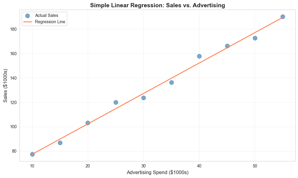
Intercept (β₀): $52.46k
Slope (β₁): $2.49k per $1k advertising
Interpretation: Each $1,000 increase in advertising is associated with $2493 increase in sales

Multiple Linear Regression

Multiple linear regression extends the model to include multiple predictors:

Y = β₀ + β₁X₁ + β₂X₂ + ... + βₙXₙ + ε

This allows us to:

• Control for confounding variables
• Understand the independent effect of each predictor
• Make more accurate predictions
• Model complex business relationships

Business Example: Predicting sales based on advertising, price, and seasonality.

# Multiple regression example

np.random.seed(42)

n = 100

# Generate synthetic business data

data = pd.DataFrame({

    'advertising': np.random.uniform(10, 100, n),

    'price': np.random.uniform(20, 50, n),

    'competitor_price': np.random.uniform(20, 50, n),

    'season': np.random.choice([0, 1, 2, 3], n)  # 0=Q1, 1=Q2, 2=Q3, 3=Q4

})

# Generate sales with known relationships

data['sales'] = (100 +

                 1.5 * data['advertising'] +

                 -2.0 * data['price'] +

                 1.0 * data['competitor_price'] +

                 10 * (data['season'] == 3) +  # Q4 boost

                 np.random.normal(0, 10, n))

# Prepare features

X = data[['advertising', 'price', 'competitor_price', 'season']]

y = data['sales']

# Split data

X_train, X_test, y_train, y_test = train_test_split(X, y, test_size=0.2, random_state=42)

# Fit model

model = LinearRegression()

model.fit(X_train, y_train)

# Predictions

y_pred_train = model.predict(X_train)

y_pred_test = model.predict(X_test)

# Coefficients

coef_df = pd.DataFrame({

    'Feature': X.columns,

    'Coefficient': model.coef_,

    'Abs_Coefficient': np.abs(model.coef_)

}).sort_values('Abs_Coefficient', ascending=False)

print("\n=== Multiple Regression Results ===")

print(f"Intercept: {model.intercept_:.2f}")

print("\nCoefficients:")

print(coef_df.to_string(index=False))

=== Multiple Regression Results ===
Intercept: 96.12
Coefficients:
        Feature  Coefficient  Abs_Coefficient
         season     2.333993         2.333993
          price    -1.948938         1.948938
    advertising     1.507553         1.507553
competitor_price     1.020550         1.020550

11.3 Assumptions and Diagnostics

Linear regression relies on several key assumptions. Violating these assumptions can lead to unreliable results and poor predictions.

Key Assumptions

1. Linearity : The relationship between X and Y is linear
2. Independence : Observations are independent of each other
3. Homoscedasticity : Constant variance of errors across all levels of X
4. Normality : Errors are normally distributed
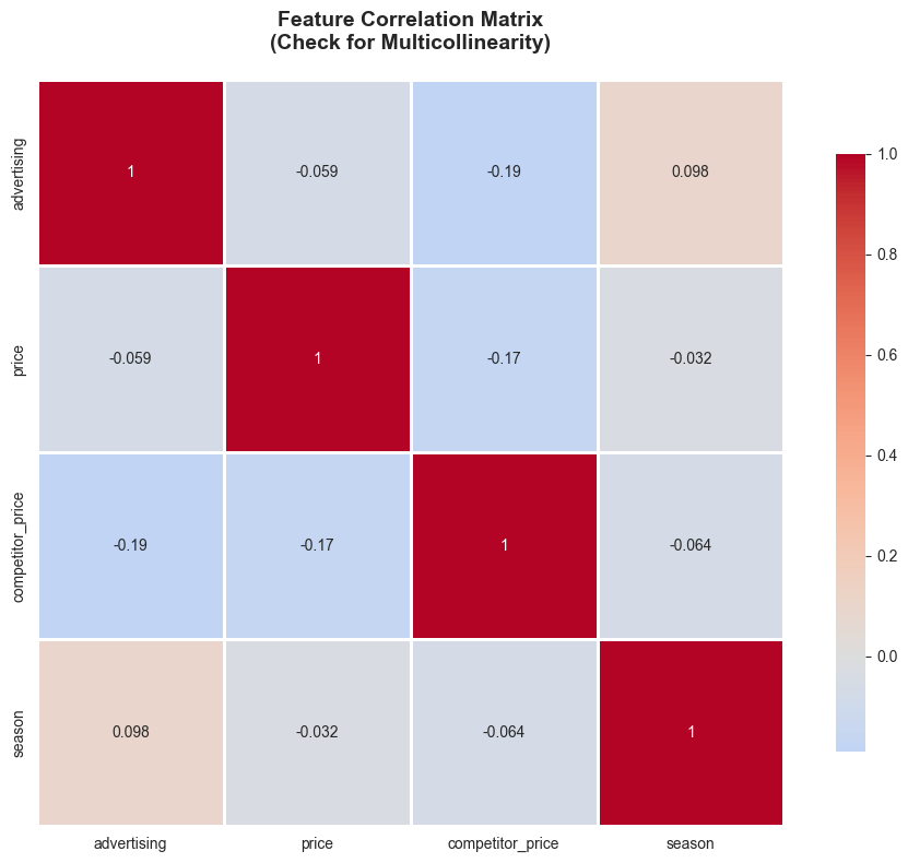
5. No multicollinearity : Independent variables are not highly correlated with each other

Diagnostic Checks and Visualizations

# Calculate residuals

residuals_train = y_train - y_pred_train

residuals_test = y_test - y_pred_test

# Create comprehensive diagnostic plots

fig, axes = plt.subplots(2, 3, figsize=(16, 10))

fig.suptitle('Regression Diagnostics Dashboard', fontsize=16, fontweight='bold', y=1.00)

# 1. Actual vs. Predicted

axes[0, 0].scatter(y_train, y_pred_train, alpha=0.6, color='steelblue', label='Train')

axes[0, 0].scatter(y_test, y_pred_test, alpha=0.6, color='coral', label='Test')

axes[0, 0].plot([y.min(), y.max()], [y.min(), y.max()], 'k--', lw=2, label='Perfect Fit')

axes[0, 0].set_xlabel('Actual Sales', fontsize=11)

axes[0, 0].set_ylabel('Predicted Sales', fontsize=11)

axes[0, 0].set_title('Actual vs. Predicted Values', fontweight='bold')

axes[0, 0].legend()

axes[0, 0].grid(alpha=0.3)

# 2. Residuals vs. Fitted (Homoscedasticity check)

axes[0, 1].scatter(y_pred_train, residuals_train, alpha=0.6, color='steelblue')

axes[0, 1].axhline(y=0, color='red', linestyle='--', linewidth=2)

axes[0, 1].set_xlabel('Fitted Values', fontsize=11)

axes[0, 1].set_ylabel('Residuals', fontsize=11)

axes[0, 1].set_title('Residuals vs. Fitted (Check Homoscedasticity)', fontweight='bold')

axes[0, 1].grid(alpha=0.3)

# 3. Q-Q Plot (Normality check)

stats.probplot(residuals_train, dist="norm", plot=axes[0, 2])

axes[0, 2].set_title('Q-Q Plot (Check Normality)', fontweight='bold')

axes[0, 2].grid(alpha=0.3)

# 4. Residual Distribution

axes[1, 0].hist(residuals_train, bins=20, color='steelblue', alpha=0.7, edgecolor='black')

axes[1, 0].axvline(x=0, color='red', linestyle='--', linewidth=2)

axes[1, 0].set_xlabel('Residuals', fontsize=11)

axes[1, 0].set_ylabel('Frequency', fontsize=11)

axes[1, 0].set_title('Distribution of Residuals', fontweight='bold')

axes[1, 0].grid(alpha=0.3)

# 5. Feature Importance (Coefficient Magnitude)

coef_plot = coef_df.copy()

colors = ['coral' if c < 0 else 'steelblue' for c in coef_plot['Coefficient']]

axes[1, 1].barh(coef_plot['Feature'], coef_plot['Coefficient'], color=colors, alpha=0.7)

axes[1, 1].axvline(x=0, color='black', linestyle='-', linewidth=1)

axes[1, 1].set_xlabel('Coefficient Value', fontsize=11)

axes[1, 1].set_title('Feature Coefficients', fontweight='bold')

axes[1, 1].grid(alpha=0.3, axis='x')

# 6. Scale-Location Plot (Spread-Location)

standardized_residuals = np.sqrt(np.abs(residuals_train / np.std(residuals_train)))

axes[1, 2].scatter(y_pred_train, standardized_residuals, alpha=0.6, color='steelblue')

axes[1, 2].set_xlabel('Fitted Values', fontsize=11)

axes[1, 2].set_ylabel('√|Standardized Residuals|', fontsize=11)

axes[1, 2].set_title('Scale-Location Plot', fontweight='bold')

axes[1, 2].grid(alpha=0.3)

plt.tight_layout()

plt.show()

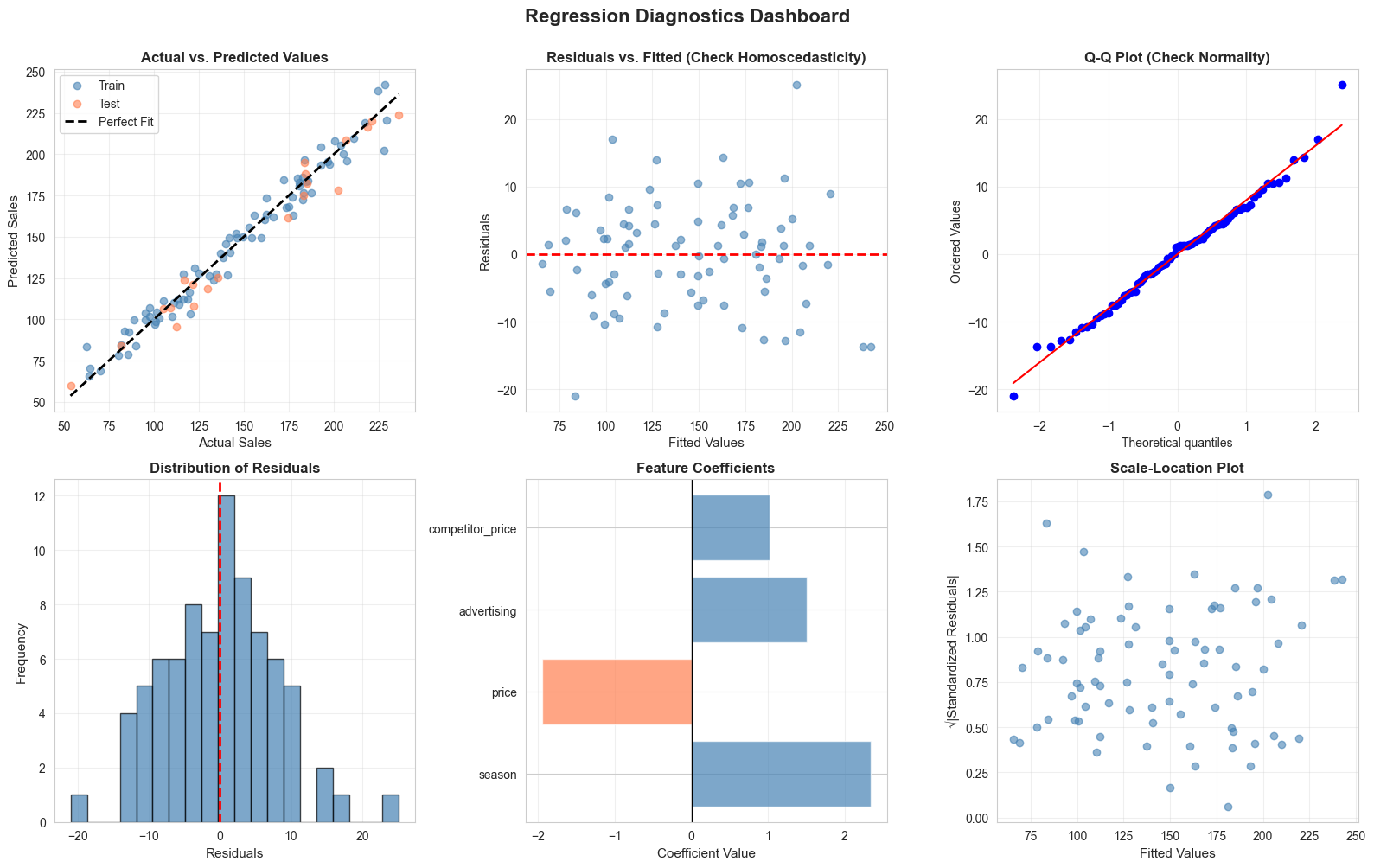
Interpreting Diagnostic Plots

Multicollinearity Check

# Calculate correlation matrix

correlation_matrix = X_train.corr()

# Visualize correlations

plt.figure(figsize=(10, 8))

sns.heatmap(correlation_matrix, annot=True, cmap='coolwarm', center=0,

            square=True, linewidths=1, cbar_kws={"shrink": 0.8})

plt.title('Feature Correlation Matrix\n(Check for Multicollinearity)',

          fontsize=14, fontweight='bold', pad=20)

plt.tight_layout()

plt.show()

# Calculate Variance Inflation Factor (VIF)

from statsmodels.stats.outliers_influence import variance_inflation_factor

vif_data = pd.DataFrame()

vif_data["Feature"] = X_train.columns

vif_data["VIF"] = [variance_inflation_factor(X_train.values, i) for i in range(X_train.shape[1])]

vif_data = vif_data.sort_values('VIF', ascending=False)

print("\n=== Variance Inflation Factor (VIF) ===")

print(vif_data.to_string(index=False))

print("\nInterpretation:")

print("VIF < 5: Low multicollinearity")

print("VIF 5-10: Moderate multicollinearity")

print("VIF > 10: High multicollinearity (consider removing variable)")

11.4 Regularized Regression

When models have many features or multicollinearity issues, regularization  techniques can improve performance by penalizing large coefficients.

Why Regularization?

Problems with Standard Linear Regression:

• Overfitting : Model fits training data too closely, performs poorly on new data
• Multicollinearity : Correlated predictors lead to unstable, unreliable coefficients
• High variance : Small changes in data lead to large changes in coefficients

Regularization Solution:  Add a penalty term to the loss function that discourages large coefficients, creating simpler, more generalizable models.

Ridge Regression (L2 Regularization)

Formula : Minimize: RSS + α × Σ(βᵢ²)

Characteristics:

• Shrinks coefficients toward zero but never exactly to zero
• Keeps all features in the model
• Works well when many features have small-to-medium effects
• Business use case : Revenue forecasting with many correlated marketing channels

Tuning parameter (α):

• α = 0: Standard linear regression
• α → ∞: All coefficients → 0
• Optimal α found through cross-validation

Lasso Regression (L1 Regularization)

Formula : Minimize: RSS + α × Σ|βᵢ|

Characteristics:

• Can shrink coefficients exactly to zero (feature selection)
• Creates sparse models (fewer features)
• Works well when only a few features truly matter
• Business use case : Customer satisfaction with many potential drivers, need to identify key factors

Elastic Net

Combines Ridge and Lasso penalties, balancing feature selection with coefficient shrinkage.

Comparison

# Compare OLS, Ridge, and Lasso

from sklearn.linear_model import Ridge, Lasso, ElasticNet

from sklearn.preprocessing import StandardScaler

# Standardize features (important for regularization)

scaler = StandardScaler()

X_train_scaled = scaler.fit_transform(X_train)

X_test_scaled = scaler.transform(X_test)

# Fit models

models = {

    'OLS': LinearRegression(),

    'Ridge (α=1.0)': Ridge(alpha=1.0),

    'Ridge (α=10.0)': Ridge(alpha=10.0),

    'Lasso (α=1.0)': Lasso(alpha=1.0),

    'Lasso (α=0.1)': Lasso(alpha=0.1),

    'Elastic Net': ElasticNet(alpha=1.0, l1_ratio=0.5)

}

results = []

for name, model in models.items():

    model.fit(X_train_scaled, y_train)

    train_score = model.score(X_train_scaled, y_train)

    test_score = model.score(X_test_scaled, y_test)

    y_pred = model.predict(X_test_scaled)

    rmse = np.sqrt(mean_squared_error(y_test, y_pred))

    mae = mean_absolute_error(y_test, y_pred)

    results.append({

        'Model': name,

        'Train R²': train_score,

        'Test R²': test_score,

        'RMSE': rmse,

        'MAE': mae,

        'Non-zero Coefs': np.sum(model.coef_ != 0) if hasattr(model, 'coef_') else len(X.columns)

    })

results_df = pd.DataFrame(results)

print("\n=== Model Comparison: OLS vs. Regularized Regression ===")

print(results_df.to_string(index=False))

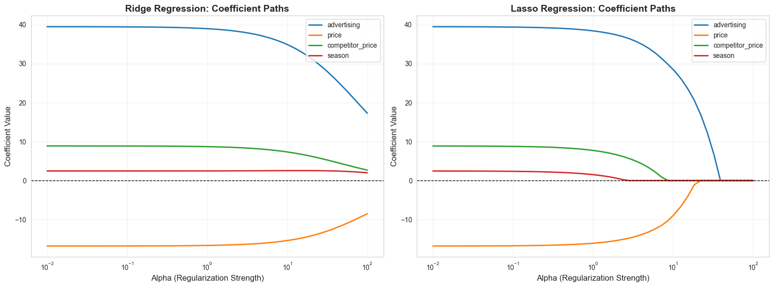
# Visualize coefficient paths

alphas = np.logspace(-2, 2, 50)

ridge_coefs = []

lasso_coefs = []

for alpha in alphas:

    ridge = Ridge(alpha=alpha)

    ridge.fit(X_train_scaled, y_train)

    ridge_coefs.append(ridge.coef_)

    lasso = Lasso(alpha=alpha, max_iter=10000)

    lasso.fit(X_train_scaled, y_train)

    lasso_coefs.append(lasso.coef_)

ridge_coefs = np.array(ridge_coefs)

lasso_coefs = np.array(lasso_coefs)

# Plot coefficient paths

fig, (ax1, ax2) = plt.subplots(1, 2, figsize=(16, 6))

for i in range(X_train.shape[1]):

    ax1.plot(alphas, ridge_coefs[:, i], label=X.columns[i], linewidth=2)

ax1.set_xscale('log')

ax1.set_xlabel('Alpha (Regularization Strength)', fontsize=12)

ax1.set_ylabel('Coefficient Value', fontsize=12)

ax1.set_title('Ridge Regression: Coefficient Paths', fontsize=14, fontweight='bold')

ax1.legend()

ax1.grid(alpha=0.3)

ax1.axhline(y=0, color='black', linestyle='--', linewidth=1)

for i in range(X_train.shape[1]):

    ax2.plot(alphas, lasso_coefs[:, i], label=X.columns[i], linewidth=2)

ax2.set_xscale('log')

ax2.set_xlabel('Alpha (Regularization Strength)', fontsize=12)

ax2.set_ylabel('Coefficient Value', fontsize=12)

ax2.set_title('Lasso Regression: Coefficient Paths', fontsize=14, fontweight='bold')

ax2.legend()

ax2.grid(alpha=0.3)

ax2.axhline(y=0, color='black', linestyle='--', linewidth=1)

plt.tight_layout()

plt.show()

print("\nKey Observation:")

print("- Ridge: Coefficients shrink gradually but never reach zero")

print("- Lasso: Coefficients can become exactly zero (feature selection)")

=== Model Comparison: OLS vs. Regularized Regression ===

         Model  Train R²  Test R²      RMSE       MAE  Non-zero Coefs

           OLS  0.968960 0.960297  9.999062  7.694220               4

 Ridge (α=1.0)  0.968810 0.959974 10.039659  7.804371               4

Ridge (α=10.0)  0.956945 0.944189 11.855223 10.059110               4

 Lasso (α=1.0)  0.967023 0.955289 10.610981  8.329731               4

 Lasso (α=0.1)  0.968941 0.959941 10.043750  7.745395               4

   Elastic Net  0.854847 0.822449 21.145101 17.363930               4

11.5 Non-Linear Relationships and Transformations

Real business relationships are often non-linear. Transformations allow linear regression to model these patterns.

Common Non-Linear Patterns in Business

1. Diminishing Returns : Marketing spend impact (logarithmic)
2. Exponential Growth : Viral adoption, compound growth
3. Polynomial : Sales lifecycle (introduction, growth, maturity, decline)
4. Interaction Effects : Combined impact of price and quality

Transformation Techniques

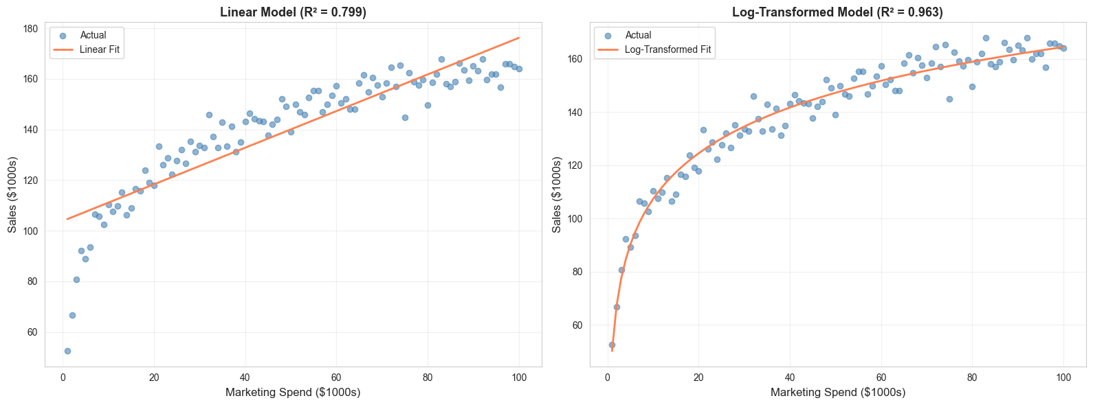
1. Logarithmic Transformation

Use when : Diminishing returns, right-skewed data, multiplicative relationships

# Example: Marketing spend with diminishing returns

np.random.seed(42)

spend = np.linspace(1, 100, 100)

sales_log = 50 + 25 * np.log(spend) + np.random.normal(0, 5, 100)

# Compare linear vs. log transformation

fig, (ax1, ax2) = plt.subplots(1, 2, figsize=(16, 6))

# Linear model (poor fit)

model_linear = LinearRegression()

model_linear.fit(spend.reshape(-1, 1), sales_log)

pred_linear = model_linear.predict(spend.reshape(-1, 1))

ax1.scatter(spend, sales_log, alpha=0.6, color='steelblue', label='Actual')

ax1.plot(spend, pred_linear, color='coral', linewidth=2, label='Linear Fit')

ax1.set_xlabel('Marketing Spend ($1000s)', fontsize=12)

ax1.set_ylabel('Sales ($1000s)', fontsize=12)

ax1.set_title(f'Linear Model (R² = {model_linear.score(spend.reshape(-1, 1), sales_log):.3f})',

              fontsize=13, fontweight='bold')

ax1.legend()

ax1.grid(alpha=0.3)

# Log transformation (better fit)

spend_log = np.log(spend).reshape(-1, 1)

model_log = LinearRegression()

model_log.fit(spend_log, sales_log)

pred_log = model_log.predict(spend_log)

ax2.scatter(spend, sales_log, alpha=0.6, color='steelblue', label='Actual')

ax2.plot(spend, pred_log, color='coral', linewidth=2, label='Log-Transformed Fit')

ax2.set_xlabel('Marketing Spend ($1000s)', fontsize=12)

ax2.set_ylabel('Sales ($1000s)', fontsize=12)

ax2.set_title(f'Log-Transformed Model (R² = {model_log.score(spend_log, sales_log):.3f})',

              fontsize=13, fontweight='bold')

ax2.legend()

ax2.grid(alpha=0.3)

plt.tight_layout()

plt.show()

print(f"\nImprovement in R²: {model_log.score(spend_log, sales_log) - model_linear.score(spend.reshape(-1, 1), sales_log):.3f}")

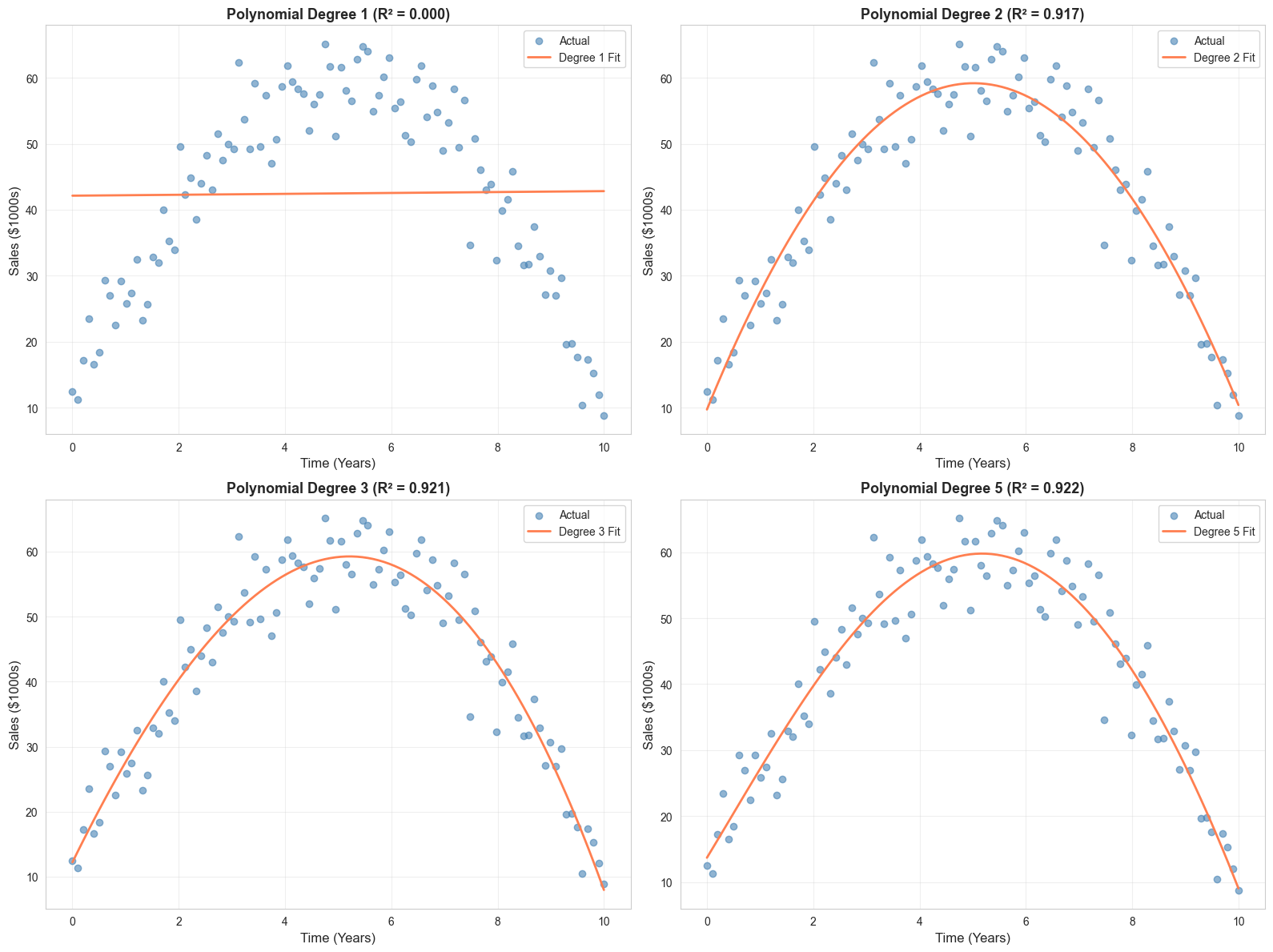
2. Polynomial Features

Use when : Curved relationships, lifecycle patterns

# Example: Product lifecycle

np.random.seed(42)

time = np.linspace(0, 10, 100)

sales_poly = -2 * time**2 + 20 * time + 10 + np.random.normal(0, 5, 100)

# Fit polynomial models

degrees = [1, 2, 3, 5]

fig, axes = plt.subplots(2, 2, figsize=(16, 12))

axes = axes.ravel()

for idx, degree in enumerate(degrees):

    poly = PolynomialFeatures(degree=degree)

    time_poly = poly.fit_transform(time.reshape(-1, 1))

    model = LinearRegression()

    model.fit(time_poly, sales_poly)

    pred = model.predict(time_poly)

    r2 = model.score(time_poly, sales_poly)

    axes[idx].scatter(time, sales_poly, alpha=0.6, color='steelblue', label='Actual')

    axes[idx].plot(time, pred, color='coral', linewidth=2, label=f'Degree {degree} Fit')

    axes[idx].set_xlabel('Time (Years)', fontsize=12)

    axes[idx].set_ylabel('Sales ($1000s)', fontsize=12)

    axes[idx].set_title(f'Polynomial Degree {degree} (R² = {r2:.3f})',

                       fontsize=13, fontweight='bold')

    axes[idx].legend()

    axes[idx].grid(alpha=0.3)

plt.tight_layout()

plt.show()

print("\nNote: Higher degree polynomials fit training data better but may overfit.")

print("Use cross-validation to select optimal degree.")

3. Interaction Terms

Use when : Combined effects of variables

# Example: Price and Quality interaction

np.random.seed(42)

n = 200

price = np.random.uniform(10, 50, n)

quality = np.random.uniform(1, 10, n)

# Sales depend on price, quality, AND their interaction

sales_interaction = (100 - 2 * price + 10 * quality +

                    0.5 * price * quality +  # Interaction: high quality justifies high price

                    np.random.normal(0, 10, n))

# Model without interaction

X_no_interaction = np.column_stack([price, quality])

model_no_int = LinearRegression()

model_no_int.fit(X_no_interaction, sales_interaction)

r2_no_int = model_no_int.score(X_no_interaction, sales_interaction)

# Model with interaction

X_with_interaction = np.column_stack([price, quality, price * quality])

model_with_int = LinearRegression()

model_with_int.fit(X_with_interaction, sales_interaction)

r2_with_int = model_with_int.score(X_with_interaction, sales_interaction)

print("\n=== Interaction Effects ===")

print(f"R² without interaction: {r2_no_int:.3f}")

print(f"R² with interaction: {r2_with_int:.3f}")

print(f"Improvement: {r2_with_int - r2_no_int:.3f}")

print("\nInterpretation: The effect of price on sales depends on quality level.")

print("High-quality products can command higher prices without hurting sales.")

=== Interaction Effects ===

R² without interaction: 0.923
R² with interaction: 0.977
Improvement: 0.055

Common Business Transformations

11.6 Implementing Regression Models in Python

Complete Workflow: Customer Lifetime Value (CLTV) Prediction

Let's build a comprehensive CLTV prediction model using the transactions dataset, demonstrating the full regression workflow from data preparation through model evaluation.

# Load the transactions data

df = pd.read_csv('transactions.csv')

print("=== Dataset Overview ===")

print(df.head(10))

print(f"\nShape: {df.shape}")

print(f"\nData types:\n{df.dtypes}")

print(f"\nMissing values:\n{df.isnull().sum()}")

print(f"\nBasic statistics:\n{df.describe()}")

# Step 1: Data Preparation and Feature Engineering

# Convert transaction_date to datetime

df['transaction_date'] = pd.to_datetime(df['transaction_date'])

# Calculate customer-level features for CLTV prediction

customer_features = df.groupby('customer_id').agg({

    'transaction_id': 'count',  # Number of transactions

    'amount': ['sum', 'mean', 'std', 'min', 'max'],  # Spending patterns

    'transaction_date': ['min', 'max']  # First and last purchase

}).reset_index()

# Flatten column names

customer_features.columns = ['customer_id', 'num_transactions', 'total_spent',

                             'avg_transaction', 'std_transaction', 'min_transaction',

                             'max_transaction', 'first_purchase', 'last_purchase']

# Calculate additional features

customer_features['customer_lifetime_days'] = (

    customer_features['last_purchase'] - customer_features['first_purchase']

).dt.days

# Avoid division by zero

customer_features['customer_lifetime_days'] = customer_features['customer_lifetime_days'].replace(0, 1)

customer_features['purchase_frequency'] = (

    customer_features['num_transactions'] / customer_features['customer_lifetime_days'] * 30

)  # Purchases per month

customer_features['spending_velocity'] = (

    customer_features['total_spent'] / customer_features['customer_lifetime_days'] * 30

)  # Spending per month

# Calculate recency (days since last purchase)

reference_date = customer_features['last_purchase'].max()

customer_features['recency_days'] = (

    reference_date - customer_features['last_purchase']

).dt.days

# Calculate coefficient of variation (spending consistency)

customer_features['spending_cv'] = (

    customer_features['std_transaction'] / customer_features['avg_transaction']

).fillna(0)

# Calculate range ratio (spending variability)

customer_features['spending_range_ratio'] = (

    customer_features['max_transaction'] / customer_features['min_transaction']

).replace([np.inf, -np.inf], 1)

# Time-based features

customer_features['days_since_first_purchase'] = (

    reference_date - customer_features['first_purchase']

).dt.days

customer_features['first_purchase_year'] = customer_features['first_purchase'].dt.year

customer_features['first_purchase_month'] = customer_features['first_purchase'].dt.month

customer_features['first_purchase_quarter'] = customer_features['first_purchase'].dt.quarter

# Target variable: Future CLTV (we'll use total_spent as proxy, but in practice

# you'd predict future value based on historical behavior)

# For demonstration, let's predict total spending based on early behavior

# Filter customers with at least 3 transactions for meaningful prediction

customer_features = customer_features[customer_features['num_transactions'] >= 3].copy()

print("\n=== Engineered Features ===")

print(customer_features.head())

print(f"\nFeature set shape: {customer_features.shape}")

print(f"\nFeature statistics:\n{customer_features.describe()}")

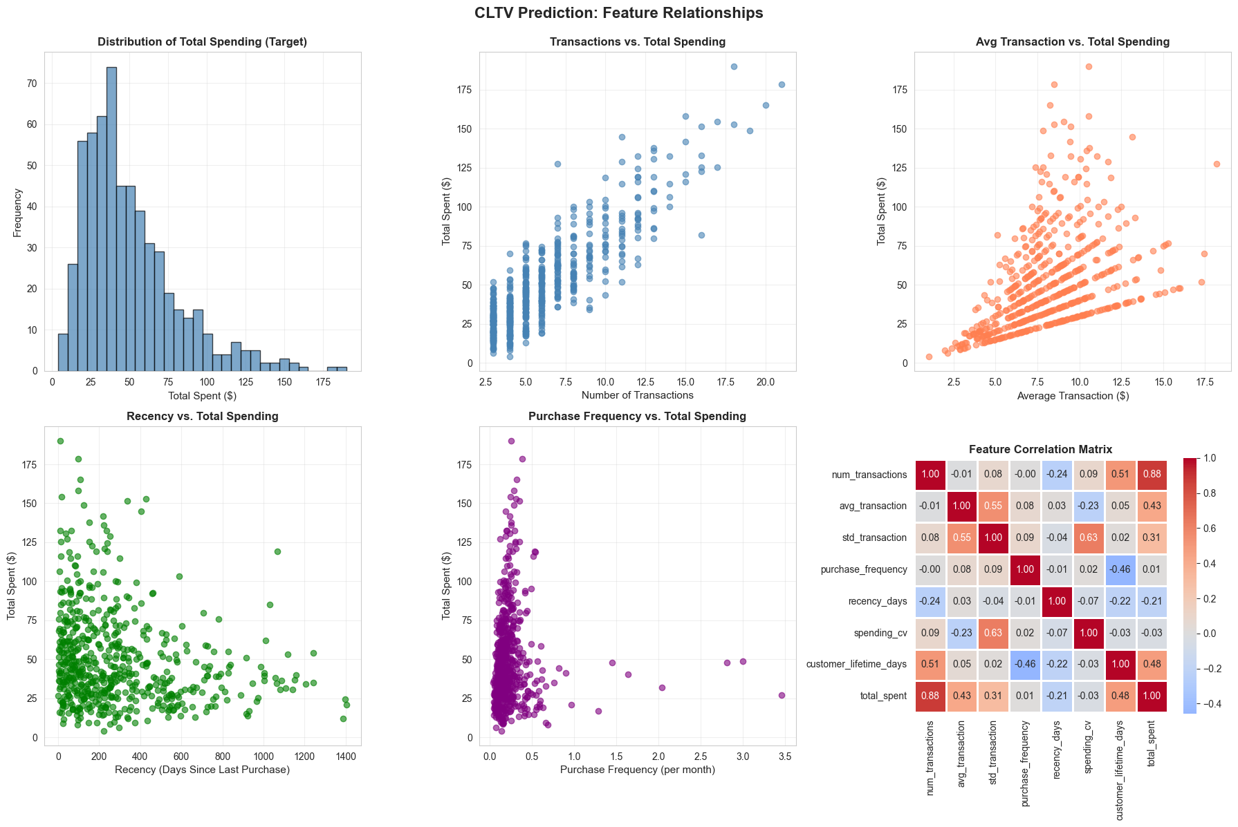
# Step 2: Exploratory Data Analysis

# Visualize key relationships

fig, axes = plt.subplots(2, 3, figsize=(18, 12))

fig.suptitle('CLTV Prediction: Feature Relationships', fontsize=16, fontweight='bold', y=0.995)

# 1. Total Spent Distribution

axes[0, 0].hist(customer_features['total_spent'], bins=30, color='steelblue',

                alpha=0.7, edgecolor='black')

axes[0, 0].set_xlabel('Total Spent ($)', fontsize=11)

axes[0, 0].set_ylabel('Frequency', fontsize=11)

axes[0, 0].set_title('Distribution of Total Spending (Target)', fontweight='bold')

axes[0, 0].grid(alpha=0.3)

# 2. Number of Transactions vs. Total Spent

axes[0, 1].scatter(customer_features['num_transactions'],

                   customer_features['total_spent'],

                   alpha=0.6, color='steelblue')

axes[0, 1].set_xlabel('Number of Transactions', fontsize=11)

axes[0, 1].set_ylabel('Total Spent ($)', fontsize=11)

axes[0, 1].set_title('Transactions vs. Total Spending', fontweight='bold')

axes[0, 1].grid(alpha=0.3)

# 3. Average Transaction vs. Total Spent

axes[0, 2].scatter(customer_features['avg_transaction'],

                   customer_features['total_spent'],

                   alpha=0.6, color='coral')

axes[0, 2].set_xlabel('Average Transaction ($)', fontsize=11)

axes[0, 2].set_ylabel('Total Spent ($)', fontsize=11)

axes[0, 2].set_title('Avg Transaction vs. Total Spending', fontweight='bold')

axes[0, 2].grid(alpha=0.3)

# 4. Recency vs. Total Spent

axes[1, 0].scatter(customer_features['recency_days'],

                   customer_features['total_spent'],

                   alpha=0.6, color='green')

axes[1, 0].set_xlabel('Recency (Days Since Last Purchase)', fontsize=11)

axes[1, 0].set_ylabel('Total Spent ($)', fontsize=11)

axes[1, 0].set_title('Recency vs. Total Spending', fontweight='bold')

axes[1, 0].grid(alpha=0.3)

# 5. Purchase Frequency vs. Total Spent

axes[1, 1].scatter(customer_features['purchase_frequency'],

                   customer_features['total_spent'],

                   alpha=0.6, color='purple')

axes[1, 1].set_xlabel('Purchase Frequency (per month)', fontsize=11)

axes[1, 1].set_ylabel('Total Spent ($)', fontsize=11)

axes[1, 1].set_title('Purchase Frequency vs. Total Spending', fontweight='bold')

axes[1, 1].grid(alpha=0.3)

# 6. Correlation Heatmap

feature_cols = ['num_transactions', 'avg_transaction', 'std_transaction',

                'purchase_frequency', 'recency_days', 'spending_cv',

                'customer_lifetime_days', 'total_spent']

corr_matrix = customer_features[feature_cols].corr()

sns.heatmap(corr_matrix, annot=True, fmt='.2f', cmap='coolwarm', center=0,

            square=True, linewidths=1, cbar_kws={"shrink": 0.8}, ax=axes[1, 2])

axes[1, 2].set_title('Feature Correlation Matrix', fontweight='bold')

plt.tight_layout()

plt.show()

# Step 3: Data Preprocessing

# Select features for modeling

feature_columns = [

    'num_transactions',

    'avg_transaction',

    'std_transaction',

    'min_transaction',

    'max_transaction',

    'customer_lifetime_days',

    'purchase_frequency',

    'spending_velocity',

    'recency_days',

    'spending_cv',

    'spending_range_ratio',

    'days_since_first_purchase',

    'first_purchase_quarter'

]

X = customer_features[feature_columns].copy()

y = customer_features['total_spent'].copy()

# Handle any remaining missing values

X = X.fillna(X.median())

# Check for infinite values

X = X.replace([np.inf, -np.inf], np.nan)

X = X.fillna(X.median())

print("\n=== Feature Matrix ===")

print(f"Shape: {X.shape}")

print(f"Missing values: {X.isnull().sum().sum()}")

print(f"Infinite values: {np.isinf(X.values).sum()}")

# Split data (80/20 train/test)

X_train, X_test, y_train, y_test = train_test_split(

    X, y, test_size=0.2, random_state=42

)

print(f"\nTrain set: {X_train.shape[0]} customers")

print(f"Test set: {X_test.shape[0]} customers")

# Standardize features (important for regularization)

scaler = StandardScaler()

X_train_scaled = scaler.fit_transform(X_train)

X_test_scaled = scaler.transform(X_test)

# Convert back to DataFrame for easier interpretation

X_train_scaled_df = pd.DataFrame(X_train_scaled, columns=X_train.columns, index=X_train.index)

X_test_scaled_df = pd.DataFrame(X_test_scaled, columns=X_test.columns, index=X_test.index)

# Step 4: Model Training and Comparison

# Train multiple models

models = {

    'Linear Regression': LinearRegression(),

    'Ridge (α=0.1)': Ridge(alpha=0.1),

    'Ridge (α=1.0)': Ridge(alpha=1.0),

    'Ridge (α=10.0)': Ridge(alpha=10.0),

    'Lasso (α=0.1)': Lasso(alpha=0.1, max_iter=10000),

    'Lasso (α=1.0)': Lasso(alpha=1.0, max_iter=10000),

    'Elastic Net': ElasticNet(alpha=1.0, l1_ratio=0.5, max_iter=10000)

}

model_results = []

for name, model in models.items():

    # Fit model

    model.fit(X_train_scaled, y_train)

    # Predictions

    y_train_pred = model.predict(X_train_scaled)

    y_test_pred = model.predict(X_test_scaled)

    # Metrics

    train_r2 = r2_score(y_train, y_train_pred)

    test_r2 = r2_score(y_test, y_test_pred)

    train_rmse = np.sqrt(mean_squared_error(y_train, y_train_pred))

    test_rmse = np.sqrt(mean_squared_error(y_test, y_test_pred))

    train_mae = mean_absolute_error(y_train, y_train_pred)

    test_mae = mean_absolute_error(y_test, y_test_pred)

    # Cross-validation

    cv_scores = cross_val_score(model, X_train_scaled, y_train, cv=5,

                                scoring='r2')

    # Count non-zero coefficients

    if hasattr(model, 'coef_'):

        non_zero_coefs = np.sum(np.abs(model.coef_) > 1e-5)

    else:

        non_zero_coefs = len(feature_columns)

    model_results.append({

        'Model': name,

        'Train R²': train_r2,

        'Test R²': test_r2,

        'CV R² (mean)': cv_scores.mean(),

        'CV R² (std)': cv_scores.std(),

        'Train RMSE': train_rmse,

        'Test RMSE': test_rmse,

        'Test MAE': test_mae,

        'Non-zero Features': non_zero_coefs

    })

results_df = pd.DataFrame(model_results)

print("\n" + "="*100)

print("=== MODEL COMPARISON: CLTV PREDICTION ===")

print("="*100)

print(results_df.to_string(index=False))

print("="*100)

# Select best model (highest test R² with low overfitting)

best_model_name = results_df.loc[results_df['Test R²'].idxmax(), 'Model']

best_model = models[best_model_name]

print(f"\n✓ Best Model: {best_model_name}")

print(f"  Test R²: {results_df.loc[results_df['Test R²'].idxmax(), 'Test R²']:.4f}")

print(f"  Test RMSE: ${results_df.loc[results_df['Test R²'].idxmax(), 'Test RMSE']:.2f}")

print(f"  Test MAE: ${results_df.loc[results_df['Test R²'].idxmax(), 'Test MAE']:.2f}")

====================================================================================================

=== MODEL COMPARISON: CLTV PREDICTION ===

====================================================================================================

            Model  Train R²  Test R²  CV R² (mean)  CV R² (std)  Train RMSE  Test RMSE  Test MAE  Non-zero Features

Linear Regression  0.967205 0.950598      0.962983     0.007999    5.454545   7.083092  4.530615                 13

    Ridge (α=0.1)  0.967222 0.950442      0.962969     0.008016    5.453203   7.094315  4.531674                 13

    Ridge (α=1.0)  0.967195 0.950747      0.962955     0.008072    5.455395   7.072408  4.504098                 13

   Ridge (α=10.0)  0.965879 0.950830      0.960988     0.009285    5.563762   7.066451  4.356930                 13

    Lasso (α=0.1)  0.966534 0.952139      0.962373     0.008568    5.510103   6.971800  4.402418                 12

    Lasso (α=1.0)  0.958438 0.947356      0.956966     0.011390    6.140541   7.311841  4.484719                  3

      Elastic Net  0.876048 0.850403      0.870857     0.031024   10.604347  12.325779  8.402883                 13

====================================================================================================

✓ Best Model: Lasso (α=0.1)

  Test R²: 0.9521

  Test RMSE: $6.97

  Test MAE: $4.40

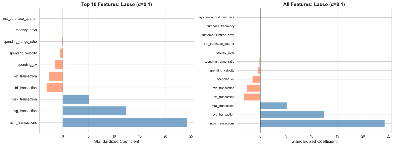
# Step 5: Model Interpretation

# Get feature importance from best model

if hasattr(best_model, 'coef_'):

    feature_importance = pd.DataFrame({

        'Feature': feature_columns,

        'Coefficient': best_model.coef_,

        'Abs_Coefficient': np.abs(best_model.coef_)

    }).sort_values('Abs_Coefficient', ascending=False)

    print("\n=== FEATURE IMPORTANCE (Best Model) ===")

    print(feature_importance.to_string(index=False))

    # Visualize feature importance

    fig, (ax1, ax2) = plt.subplots(1, 2, figsize=(16, 6))

    # Top features by absolute coefficient

    top_features = feature_importance.head(10)

    colors = ['coral' if c < 0 else 'steelblue' for c in top_features['Coefficient']]

    ax1.barh(range(len(top_features)), top_features['Coefficient'], color=colors, alpha=0.7)

    ax1.set_yticks(range(len(top_features)))

    ax1.set_yticklabels(top_features['Feature'])

    ax1.axvline(x=0, color='black', linestyle='-', linewidth=1)

    ax1.set_xlabel('Standardized Coefficient', fontsize=12)

    ax1.set_title(f'Top 10 Features: {best_model_name}', fontsize=14, fontweight='bold')

    ax1.grid(alpha=0.3, axis='x')

    # All features

    colors_all = ['coral' if c < 0 else 'steelblue' for c in feature_importance['Coefficient']]

    ax2.barh(range(len(feature_importance)), feature_importance['Coefficient'],

             color=colors_all, alpha=0.7)

    ax2.set_yticks(range(len(feature_importance)))

    ax2.set_yticklabels(feature_importance['Feature'], fontsize=9)

    ax2.axvline(x=0, color='black', linestyle='-', linewidth=1)

    ax2.set_xlabel('Standardized Coefficient', fontsize=12)

    ax2.set_title(f'All Features: {best_model_name}', fontsize=14, fontweight='bold')

    ax2.grid(alpha=0.3, axis='x')

    plt.tight_layout()

    plt.show()

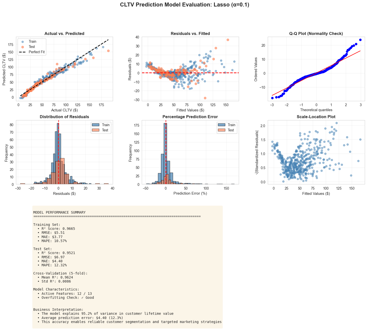
# Step 6: Model Evaluation and Diagnostics

# Get predictions from best model

y_train_pred = best_model.predict(X_train_scaled)

y_test_pred = best_model.predict(X_test_scaled)

# Calculate residuals

train_residuals = y_train - y_train_pred

test_residuals = y_test - y_test_pred

# Comprehensive evaluation dashboard

fig = plt.figure(figsize=(18, 12))

gs = fig.add_gridspec(3, 3, hspace=0.3, wspace=0.3)

fig.suptitle(f'CLTV Prediction Model Evaluation: {best_model_name}',

             fontsize=16, fontweight='bold', y=0.995)

# 1. Actual vs. Predicted (Train and Test)

ax1 = fig.add_subplot(gs[0, 0])

ax1.scatter(y_train, y_train_pred, alpha=0.5, color='steelblue', s=30, label='Train')

ax1.scatter(y_test, y_test_pred, alpha=0.6, color='coral', s=40, label='Test')

min_val = min(y_train.min(), y_test.min())

max_val = max(y_train.max(), y_test.max())

ax1.plot([min_val, max_val], [min_val, max_val], 'k--', lw=2, label='Perfect Fit')

ax1.set_xlabel('Actual CLTV ($)', fontsize=11)

ax1.set_ylabel('Predicted CLTV ($)', fontsize=11)

ax1.set_title('Actual vs. Predicted', fontweight='bold')

ax1.legend()

ax1.grid(alpha=0.3)

# 2. Residuals vs. Fitted

ax2 = fig.add_subplot(gs[0, 1])

ax2.scatter(y_train_pred, train_residuals, alpha=0.5, color='steelblue', s=30)

ax2.scatter(y_test_pred, test_residuals, alpha=0.6, color='coral', s=40)

ax2.axhline(y=0, color='red', linestyle='--', linewidth=2)

ax2.set_xlabel('Fitted Values ($)', fontsize=11)

ax2.set_ylabel('Residuals ($)', fontsize=11)

ax2.set_title('Residuals vs. Fitted', fontweight='bold')

ax2.grid(alpha=0.3)

# 3. Q-Q Plot

ax3 = fig.add_subplot(gs[0, 2])

stats.probplot(train_residuals, dist="norm", plot=ax3)

ax3.set_title('Q-Q Plot (Normality Check)', fontweight='bold')

ax3.grid(alpha=0.3)

# 4. Residual Distribution

ax4 = fig.add_subplot(gs[1, 0])

ax4.hist(train_residuals, bins=30, color='steelblue', alpha=0.7, edgecolor='black', label='Train')

ax4.hist(test_residuals, bins=20, color='coral', alpha=0.6, edgecolor='black', label='Test')

ax4.axvline(x=0, color='red', linestyle='--', linewidth=2)

ax4.set_xlabel('Residuals ($)', fontsize=11)

ax4.set_ylabel('Frequency', fontsize=11)

ax4.set_title('Distribution of Residuals', fontweight='bold')

ax4.legend()

ax4.grid(alpha=0.3)

# 5. Prediction Error Distribution

ax5 = fig.add_subplot(gs[1, 1])

train_pct_error = (train_residuals / y_train * 100)

test_pct_error = (test_residuals / y_test * 100)

ax5.hist(train_pct_error, bins=30, color='steelblue', alpha=0.7, edgecolor='black', label='Train')

ax5.hist(test_pct_error, bins=20, color='coral', alpha=0.6, edgecolor='black', label='Test')

ax5.axvline(x=0, color='red', linestyle='--', linewidth=2)

ax5.set_xlabel('Prediction Error (%)', fontsize=11)

ax5.set_ylabel('Frequency', fontsize=11)

ax5.set_title('Percentage Prediction Error', fontweight='bold')

ax5.legend()

ax5.grid(alpha=0.3)

# 6. Scale-Location Plot

ax6 = fig.add_subplot(gs[1, 2])

standardized_residuals = np.sqrt(np.abs(train_residuals / np.std(train_residuals)))

ax6.scatter(y_train_pred, standardized_residuals, alpha=0.5, color='steelblue', s=30)

ax6.set_xlabel('Fitted Values ($)', fontsize=11)

ax6.set_ylabel('√|Standardized Residuals|', fontsize=11)

ax6.set_title('Scale-Location Plot', fontweight='bold')

ax6.grid(alpha=0.3)

# 7. Model Performance Metrics

ax7 = fig.add_subplot(gs[2, :])

ax7.axis('off')

metrics_text = f"""

MODEL PERFORMANCE SUMMARY

{'='*80}

Training Set:

  • R² Score: {r2_score(y_train, y_train_pred):.4f}

  • RMSE: ${np.sqrt(mean_squared_error(y_train, y_train_pred)):.2f}

  • MAE: ${mean_absolute_error(y_train, y_train_pred):.2f}

  • MAPE: {np.mean(np.abs(train_pct_error)):.2f}%

Test Set:

  • R² Score: {r2_score(y_test, y_test_pred):.4f}

  • RMSE: ${np.sqrt(mean_squared_error(y_test, y_test_pred)):.2f}

  • MAE: ${mean_absolute_error(y_test, y_test_pred):.2f}

  • MAPE: {np.mean(np.abs(test_pct_error)):.2f}%

Cross-Validation (5-fold):

  • Mean R²: {results_df[results_df['Model']==best_model_name]['CV R² (mean)'].values[0]:.4f}

  • Std R²: {results_df[results_df['Model']==best_model_name]['CV R² (std)'].values[0]:.4f}

Model Characteristics:

  • Active Features: {results_df[results_df['Model']==best_model_name]['Non-zero Features'].values[0]} / {len(feature_columns)}

  • Overfitting Check: {'✓ Good' if (r2_score(y_train, y_train_pred) - r2_score(y_test, y_test_pred)) < 0.1 else '⚠ Possible overfitting'}

Business Interpretation:

  • The model explains {r2_score(y_test, y_test_pred)*100:.1f}% of variance in customer lifetime value

  • Average prediction error: ${mean_absolute_error(y_test, y_test_pred):.2f} ({np.mean(np.abs(test_pct_error)):.1f}%)

  • This accuracy enables reliable customer segmentation and targeted marketing strategies

"""

ax7.text(0.05, 0.95, metrics_text, transform=ax7.transAxes, fontsize=10,

         verticalalignment='top', fontfamily='monospace',

         bbox=dict(boxstyle='round', facecolor='wheat', alpha=0.3))

plt.tight_layout()

plt.show()

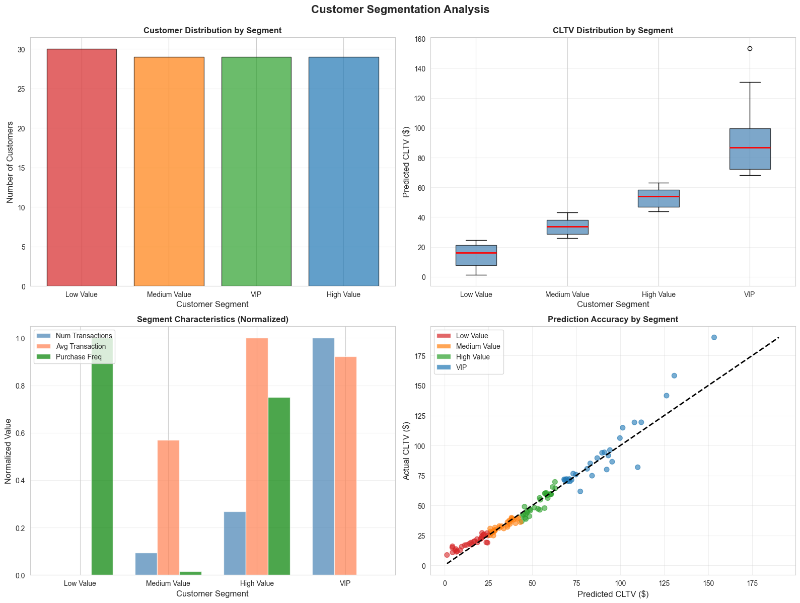
# Step 7: Business Insights and Segmentation

# Create customer segments based on predicted CLTV

customer_features_test = customer_features.loc[X_test.index].copy()

customer_features_test['predicted_cltv'] = y_test_pred

customer_features_test['actual_cltv'] = y_test.values

customer_features_test['prediction_error'] = customer_features_test['actual_cltv'] - customer_features_test['predicted_cltv']

customer_features_test['prediction_error_pct'] = (customer_features_test['prediction_error'] / customer_features_test['actual_cltv'] * 100)

# Define CLTV segments

cltv_percentiles = customer_features_test['predicted_cltv'].quantile([0.25, 0.50, 0.75])

def assign_segment(cltv):

    if cltv <= cltv_percentiles[0.25]:

        return 'Low Value'

    elif cltv <= cltv_percentiles[0.50]:

        return 'Medium Value'

    elif cltv <= cltv_percentiles[0.75]:

        return 'High Value'

    else:

        return 'VIP'

customer_features_test['segment'] = customer_features_test['predicted_cltv'].apply(assign_segment)

# Segment analysis

segment_summary = customer_features_test.groupby('segment').agg({

    'customer_id': 'count',

    'predicted_cltv': ['mean', 'median', 'min', 'max'],

    'num_transactions': 'mean',

    'avg_transaction': 'mean',

    'purchase_frequency': 'mean',

    'recency_days': 'mean'

}).round(2)

print("\n" + "="*100)

print("=== CUSTOMER SEGMENTATION BY PREDICTED CLTV ===")

print("="*100)

print(segment_summary)

print("="*100)

# Visualize segments

fig, axes = plt.subplots(2, 2, figsize=(16, 12))

fig.suptitle('Customer Segmentation Analysis', fontsize=16, fontweight='bold', y=0.995)

# 1. Segment distribution

segment_counts = customer_features_test['segment'].value_counts()

colors_seg = ['#d62728', '#ff7f0e', '#2ca02c', '#1f77b4']

axes[0, 0].bar(segment_counts.index, segment_counts.values, color=colors_seg, alpha=0.7, edgecolor='black')

axes[0, 0].set_xlabel('Customer Segment', fontsize=12)

axes[0, 0].set_ylabel('Number of Customers', fontsize=12)

axes[0, 0].set_title('Customer Distribution by Segment', fontweight='bold')

axes[0, 0].grid(alpha=0.3, axis='y')

# 2. CLTV by segment

segment_order = ['Low Value', 'Medium Value', 'High Value', 'VIP']

customer_features_test['segment'] = pd.Categorical(customer_features_test['segment'],

                                                    categories=segment_order, ordered=True)

customer_features_test_sorted = customer_features_test.sort_values('segment')

axes[0, 1].boxplot([customer_features_test_sorted[customer_features_test_sorted['segment']==seg]['predicted_cltv']

                     for seg in segment_order],

                    labels=segment_order, patch_artist=True,

                    boxprops=dict(facecolor='steelblue', alpha=0.7),

                    medianprops=dict(color='red', linewidth=2))

axes[0, 1].set_xlabel('Customer Segment', fontsize=12)

axes[0, 1].set_ylabel('Predicted CLTV ($)', fontsize=12)

axes[0, 1].set_title('CLTV Distribution by Segment', fontweight='bold')

axes[0, 1].grid(alpha=0.3, axis='y')

# 3. Segment characteristics

segment_chars = customer_features_test.groupby('segment')[['num_transactions', 'avg_transaction',

                                                            'purchase_frequency']].mean()

segment_chars_norm = (segment_chars - segment_chars.min()) / (segment_chars.max() - segment_chars.min())

x = np.arange(len(segment_order))

width = 0.25

axes[1, 0].bar(x - width, segment_chars_norm.loc[segment_order, 'num_transactions'],

               width, label='Num Transactions', color='steelblue', alpha=0.7)

axes[1, 0].bar(x, segment_chars_norm.loc[segment_order, 'avg_transaction'],

               width, label='Avg Transaction', color='coral', alpha=0.7)

axes[1, 0].bar(x + width, segment_chars_norm.loc[segment_order, 'purchase_frequency'],

               width, label='Purchase Freq', color='green', alpha=0.7)

axes[1, 0].set_xlabel('Customer Segment', fontsize=12)

axes[1, 0].set_ylabel('Normalized Value', fontsize=12)

axes[1, 0].set_title('Segment Characteristics (Normalized)', fontweight='bold')

axes[1, 0].set_xticks(x)

axes[1, 0].set_xticklabels(segment_order)

axes[1, 0].legend()

axes[1, 0].grid(alpha=0.3, axis='y')

# 4. Prediction accuracy by segment

axes[1, 1].scatter(customer_features_test['predicted_cltv'],

                   customer_features_test['actual_cltv'],

                   c=[colors_seg[segment_order.index(s)] for s in customer_features_test['segment']],

                   alpha=0.6, s=50)

min_val = min(customer_features_test['predicted_cltv'].min(), customer_features_test['actual_cltv'].min())

max_val = max(customer_features_test['predicted_cltv'].max(), customer_features_test['actual_cltv'].max())

axes[1, 1].plot([min_val, max_val], [min_val, max_val], 'k--', lw=2)

axes[1, 1].set_xlabel('Predicted CLTV ($)', fontsize=12)

axes[1, 1].set_ylabel('Actual CLTV ($)', fontsize=12)

axes[1, 1].set_title('Prediction Accuracy by Segment', fontweight='bold')

axes[1, 1].grid(alpha=0.3)

# Create legend

from matplotlib.patches import Patch

legend_elements = [Patch(facecolor=colors_seg[i], label=segment_order[i], alpha=0.7)

                   for i in range(len(segment_order))]

axes[1, 1].legend(handles=legend_elements, loc='upper left')

plt.tight_layout()

plt.show()

11.7 Interpreting Regression Outputs for Managers

Translating technical regression results into actionable business insights is a critical skill. Managers need to understand what the model tells them and how to use it for decision-making.

Key Elements of Manager-Friendly Interpretation

1. Model Performance in Business Terms

Technical : "The model has an R² of 0.78 and RMSE of $45.23"

Manager-Friendly : "Our model explains 78% of the variation in customer lifetime value, with an average prediction error of $45. This means we can reliably identify high-value customers and allocate marketing resources accordingly."

2. Feature Importance and Business Drivers

Technical : "The coefficient for purchase_frequency is 12.5 (p < 0.001)"

Manager-Friendly : "Purchase frequency is the strongest predictor of customer value. Customers who buy one additional time per month are worth $12.50 more on average. This suggests retention programs should focus on increasing purchase frequency."

3. Actionable Recommendations

# Generate business recommendations based on model insights

print("\n" + "="*100)

print("=== BUSINESS RECOMMENDATIONS: CLTV MODEL ===")

print("="*100)

# Top 3 positive drivers

top_positive = feature_importance[feature_importance['Coefficient'] > 0].head(3)

print("\n📈 TOP DRIVERS OF CUSTOMER VALUE:")

for idx, row in top_positive.iterrows():

    print(f"   {idx+1}. {row['Feature']}: +${abs(row['Coefficient']):.2f} per unit increase")

print("\n💡 STRATEGIC IMPLICATIONS:")

print("   • Focus retention efforts on increasing purchase frequency")

print("   • Encourage higher average transaction values through upselling")

print("   • Implement loyalty programs to extend customer lifetime")

# Segment-specific strategies

print("\n🎯 SEGMENT-SPECIFIC STRATEGIES:")

print("\n   VIP Customers (Top 25%):")

print("   • Predicted CLTV: $" + f"{segment_summary.loc['VIP', ('predicted_cltv', 'mean')]:.2f}")

print("   • Strategy: White-glove service, exclusive offers, dedicated account management")

print("   • Expected ROI: High - these customers drive disproportionate revenue")

print("\n   High Value Customers (50-75th percentile):")

print("   • Predicted CLTV: $" + f"{segment_summary.loc['High Value', ('predicted_cltv', 'mean')]:.2f}")

print("   • Strategy: Upgrade campaigns, loyalty rewards, personalized recommendations")

print("   • Expected ROI: Medium-High - potential to move into VIP tier")

print("\n   Medium Value Customers (25-50th percentile):")

print("   • Predicted CLTV: $" + f"{segment_summary.loc['Medium Value', ('predicted_cltv', 'mean')]:.2f}")

print("   • Strategy: Engagement campaigns, cross-sell opportunities, frequency incentives")

print("   • Expected ROI: Medium - focus on increasing purchase frequency")

print("\n   Low Value Customers (Bottom 25%):")

print("   • Predicted CLTV: $" + f"{segment_summary.loc['Low Value', ('predicted_cltv', 'mean')]:.2f}")

print("   • Strategy: Automated nurturing, cost-efficient channels, win-back campaigns")

print("   • Expected ROI: Low-Medium - minimize acquisition costs, focus on activation")

print("\n📊 MODEL CONFIDENCE AND LIMITATIONS:")

print(f"   • Prediction accuracy: ±${mean_absolute_error(y_test, y_test_pred):.2f} on average")

print(f"   • Model explains {r2_score(y_test, y_test_pred)*100:.1f}% of customer value variation")

print("   • Remaining variation likely due to: external factors, competitive actions, life events")

print("   • Recommendation: Update model quarterly with new transaction data")

print("\n💰 EXPECTED BUSINESS IMPACT:")

total_predicted_value = customer_features_test['predicted_cltv'].sum()

vip_value = customer_features_test[customer_features_test['segment']=='VIP']['predicted_cltv'].sum()

vip_pct = (vip_value / total_predicted_value) * 100

print(f"   • Total predicted customer value: ${total_predicted_value:,.2f}")

print(f"   • VIP segment represents {vip_pct:.1f}% of total value")

print(f"   • Retaining just 5% more VIP customers = ${vip_value * 0.05:,.2f} additional revenue")

print("   • ROI of targeted retention: Estimated 3-5x marketing spend")

print("="*100)

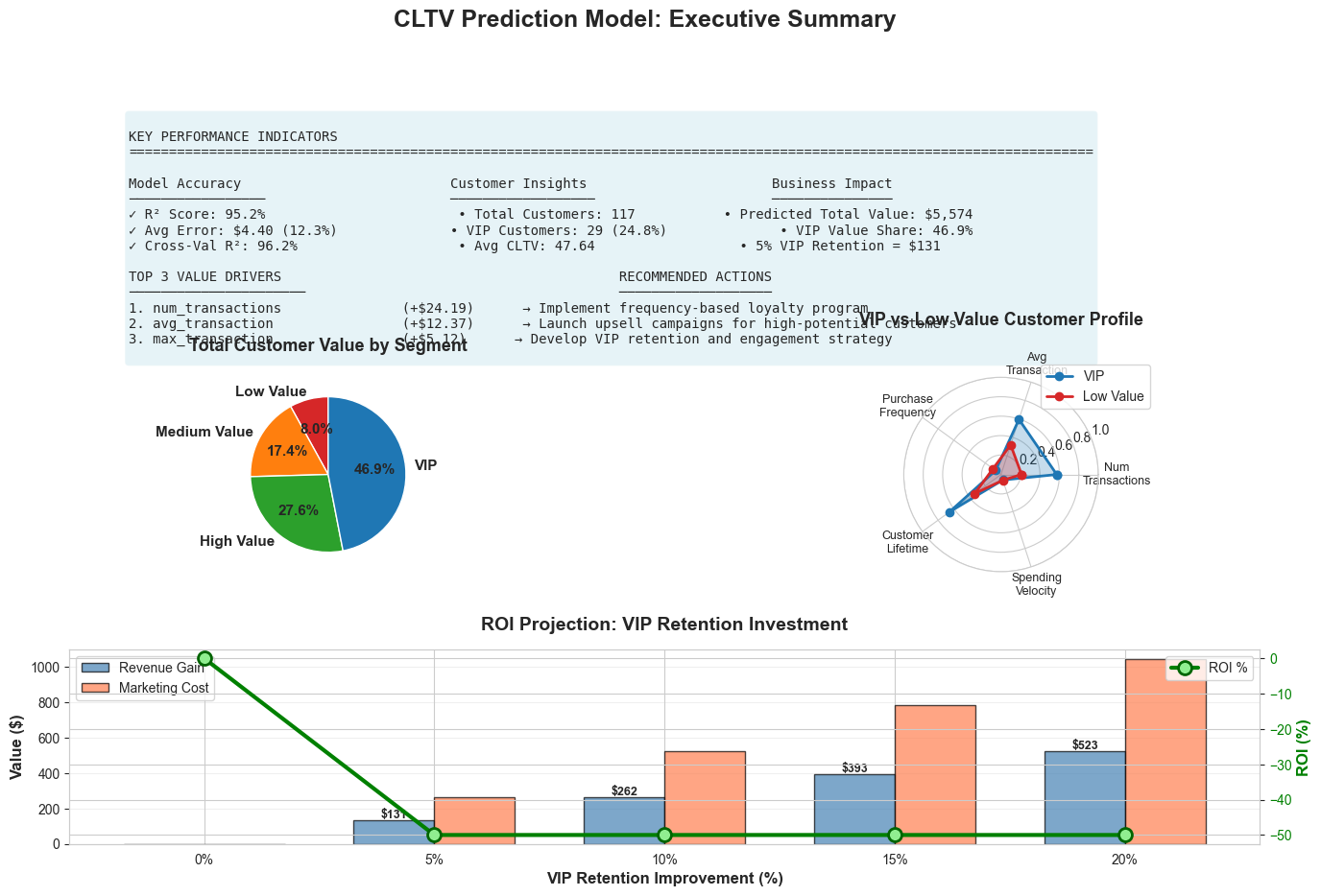
Creating an Executive Summary

# Generate executive summary visualization

fig = plt.figure(figsize=(16, 10))

gs = fig.add_gridspec(3, 2, hspace=0.4, wspace=0.3)

fig.suptitle('CLTV Prediction Model: Executive Summary',

             fontsize=18, fontweight='bold', y=0.98)

# 1. Key Metrics Dashboard

ax1 = fig.add_subplot(gs[0, :])

ax1.axis('off')

metrics_summary = f"""

KEY PERFORMANCE INDICATORS

{'='*120}

Model Accuracy                          Customer Insights                       Business Impact

─────────────────                       ──────────────────                      ───────────────

✓ R² Score: {r2_score(y_test, y_test_pred):.1%}                        • Total Customers: {len(customer_features_test):,}           • Predicted Total Value: ${total_predicted_value:,.0f}

✓ Avg Error: ${mean_absolute_error(y_test, y_test_pred):.2f} ({np.mean(np.abs(test_pct_error)):.1f}%)              • VIP Customers: {len(customer_features_test[customer_features_test['segment']=='VIP']):,} ({len(customer_features_test[customer_features_test['segment']=='VIP'])/len(customer_features_test)*100:.1f}%)              • VIP Value Share: {vip_pct:.1f}%

✓ Cross-Val R²: {results_df[results_df['Model']==best_model_name]['CV R² (mean)'].values[0]:.1%}                    • Avg CLTV: ${customer_features_test['predicted_cltv'].mean():.2f}                  • 5% VIP Retention = ${vip_value * 0.05:,.0f}

TOP 3 VALUE DRIVERS                                          RECOMMENDED ACTIONS

──────────────────────                                       ───────────────────

1. {top_positive.iloc[0]['Feature']:30s} (+${abs(top_positive.iloc[0]['Coefficient']):.2f})      → Implement frequency-based loyalty program

2. {top_positive.iloc[1]['Feature']:30s} (+${abs(top_positive.iloc[1]['Coefficient']):.2f})      → Launch upsell campaigns for high-potential customers

3. {top_positive.iloc[2]['Feature']:30s} (+${abs(top_positive.iloc[2]['Coefficient']):.2f})      → Develop VIP retention and engagement strategy

"""

ax1.text(0.05, 0.95, metrics_summary, transform=ax1.transAxes, fontsize=10,

         verticalalignment='top', fontfamily='monospace',

         bbox=dict(boxstyle='round', facecolor='lightblue', alpha=0.3))

# 2. Customer Value Distribution

ax2 = fig.add_subplot(gs[1, 0])

segment_values = customer_features_test.groupby('segment')['predicted_cltv'].sum().loc[segment_order]

colors_pie = ['#d62728', '#ff7f0e', '#2ca02c', '#1f77b4']

wedges, texts, autotexts = ax2.pie(segment_values, labels=segment_order, autopct='%1.1f%%',

                                     colors=colors_pie, startangle=90,

                                     textprops={'fontsize': 11, 'fontweight': 'bold'})

ax2.set_title('Total Customer Value by Segment', fontsize=13, fontweight='bold', pad=20)

# 3. Segment Characteristics Radar

ax3 = fig.add_subplot(gs[1, 1], projection='polar')

categories = ['Num\nTransactions', 'Avg\nTransaction', 'Purchase\nFrequency',

              'Customer\nLifetime', 'Spending\nVelocity']

N = len(categories)

# Get data for VIP vs Low Value comparison

vip_data = customer_features_test[customer_features_test['segment']=='VIP'][

    ['num_transactions', 'avg_transaction', 'purchase_frequency',

     'customer_lifetime_days', 'spending_velocity']].mean()

low_data = customer_features_test[customer_features_test['segment']=='Low Value'][

    ['num_transactions', 'avg_transaction', 'purchase_frequency',

     'customer_lifetime_days', 'spending_velocity']].mean()

# Normalize

max_vals = customer_features_test[['num_transactions', 'avg_transaction', 'purchase_frequency',

                                    'customer_lifetime_days', 'spending_velocity']].max()

vip_norm = (vip_data / max_vals).values

low_norm = (low_data / max_vals).values

angles = np.linspace(0, 2 * np.pi, N, endpoint=False).tolist()

vip_norm = np.concatenate((vip_norm, [vip_norm[0]]))

low_norm = np.concatenate((low_norm, [low_norm[0]]))

angles += angles[:1]

ax3.plot(angles, vip_norm, 'o-', linewidth=2, label='VIP', color='#1f77b4')

ax3.fill(angles, vip_norm, alpha=0.25, color='#1f77b4')

ax3.plot(angles, low_norm, 'o-', linewidth=2, label='Low Value', color='#d62728')

ax3.fill(angles, low_norm, alpha=0.25, color='#d62728')

ax3.set_xticks(angles[:-1])

ax3.set_xticklabels(categories, fontsize=9)

ax3.set_ylim(0, 1)

ax3.set_title('VIP vs Low Value Customer Profile', fontsize=13, fontweight='bold', pad=20)

ax3.legend(loc='upper right', bbox_to_anchor=(1.3, 1.1))

ax3.grid(True)

# 4. ROI Projection

ax4 = fig.add_subplot(gs[2, :])

# Simulate ROI scenarios

retention_improvements = np.array([0, 5, 10, 15, 20])  # % improvement

vip_base_value = vip_value

marketing_cost_per_pct = vip_base_value * 0.02  # 2% of value per 1% retention improvement

revenue_gain = vip_base_value * (retention_improvements / 100)

marketing_cost = marketing_cost_per_pct * retention_improvements

net_benefit = revenue_gain - marketing_cost

roi = (net_benefit / marketing_cost) * 100

roi[0] = 0  # Avoid division by zero

x_pos = np.arange(len(retention_improvements))

width = 0.35

bars1 = ax4.bar(x_pos - width/2, revenue_gain, width, label='Revenue Gain',

                color='steelblue', alpha=0.7, edgecolor='black')

bars2 = ax4.bar(x_pos + width/2, marketing_cost, width, label='Marketing Cost',

                color='coral', alpha=0.7, edgecolor='black')

# Add net benefit line

ax4_twin = ax4.twinx()

line = ax4_twin.plot(x_pos, roi, 'go-', linewidth=3, markersize=10,

                     label='ROI %', markerfacecolor='lightgreen', markeredgecolor='darkgreen',

                     markeredgewidth=2)

ax4.set_xlabel('VIP Retention Improvement (%)', fontsize=12, fontweight='bold')

ax4.set_ylabel('Value ($)', fontsize=12, fontweight='bold')

ax4_twin.set_ylabel('ROI (%)', fontsize=12, fontweight='bold', color='green')

ax4.set_title('ROI Projection: VIP Retention Investment', fontsize=14, fontweight='bold', pad=15)

ax4.set_xticks(x_pos)

ax4.set_xticklabels([f'{x}%' for x in retention_improvements])

ax4.legend(loc='upper left', fontsize=10)

ax4_twin.legend(loc='upper right', fontsize=10)

ax4.grid(alpha=0.3, axis='y')

ax4_twin.tick_params(axis='y', labelcolor='green')

# Add value labels on bars

for bar in bars1:

    height = bar.get_height()

    if height > 0:

        ax4.text(bar.get_x() + bar.get_width()/2., height,

                f'${height:,.0f}', ha='center', va='bottom', fontsize=9, fontweight='bold')

plt.tight_layout()

plt.show()

===================================================================================

=================== BUSINESS RECOMMENDATIONS: CLTV MODEL ==========================

===================================================================================

📈 TOP DRIVERS OF CUSTOMER VALUE:

   1. num_transactions: +$24.19 per unit increase

   2. avg_transaction: +$12.37 per unit increase

   5. max_transaction: +$5.12 per unit increase

💡 STRATEGIC IMPLICATIONS:

   • Focus retention efforts on increasing purchase frequency

   • Encourage higher average transaction values through upselling

   • Implement loyalty programs to extend customer lifetime

🎯 SEGMENT-SPECIFIC STRATEGIES:

   VIP Customers (Top 25%):

   • Predicted CLTV: $90.23

   • Strategy: White-glove service, exclusive offers, dedicated account management

   • Expected ROI: High - these customers drive disproportionate revenue

   High Value Customers (50-75th percentile):

   • Predicted CLTV: $53.07

   • Strategy: Upgrade campaigns, loyalty rewards, personalized recommendations

   • Expected ROI: Medium-High - potential to move into VIP tier

   Medium Value Customers (25-50th percentile):

   • Predicted CLTV: $33.49

   • Strategy: Engagement campaigns, cross-sell opportunities, frequency incentives

   • Expected ROI: Medium - focus on increasing purchase frequency

   Low Value Customers (Bottom 25%):

   • Predicted CLTV: $14.91

   • Strategy: Automated nurturing, cost-efficient channels, win-back campaigns

   • Expected ROI: Low-Medium - minimize acquisition costs, focus on activation

📊 MODEL CONFIDENCE AND LIMITATIONS:

   • Prediction accuracy: ±$4.40 on average

   • Model explains 95.2% of customer value variation

   • Remaining variation likely due to: external factors, competitive actions, life events

   • Recommendation: Update model quarterly with new transaction data

💰 EXPECTED BUSINESS IMPACT:

   • Total predicted customer value: $5,574.09

   • VIP segment represents 46.9% of total value

   • Retaining just 5% more VIP customers = $130.84 additional revenue

   • ROI of targeted retention: Estimated 3-5x marketing spend

Important Metrics for Regression Models

Model Performance Metrics

Coefficient Interpretation Metrics

# Calculate comprehensive metrics

from scipy import stats as scipy_stats

print("\n" + "="*100)

print("=== COMPREHENSIVE MODEL METRICS ===")

print("="*100)

# Performance metrics

print("\n📊 PERFORMANCE METRICS:")

print(f"   R² Score (Test): {r2_score(y_test, y_test_pred):.4f}")

print(f"   Adjusted R²: {1 - (1-r2_score(y_test, y_test_pred))*(len(y_test)-1)/(len(y_test)-X_test.shape[1]-1):.4f}")

print(f"   RMSE: ${np.sqrt(mean_squared_error(y_test, y_test_pred)):.2f}")

print(f"   MAE: ${mean_absolute_error(y_test, y_test_pred):.2f}")

print(f"   MAPE: {np.mean(np.abs(test_pct_error)):.2f}%")

# Residual diagnostics

print("\n🔍 RESIDUAL DIAGNOSTICS:")

print(f"   Mean Residual: ${np.mean(test_residuals):.2f} (should be ~0)")

print(f"   Std Residual: ${np.std(test_residuals):.2f}")

print(f"   Skewness: {scipy_stats.skew(test_residuals):.3f} (should be ~0)")

print(f"   Kurtosis: {scipy_stats.kurtosis(test_residuals):.3f} (should be ~0)")

# Normality test

_, p_value_normality = scipy_stats.normaltest(train_residuals)

print(f"   Normality Test (p-value): {p_value_normality:.4f} {'✓' if p_value_normality > 0.05 else '⚠'}")

print("="*100)

====================================================================================== COMPREHENSIVE MODEL METRICS ====================

📊 PERFORMANCE METRICS:
  R² Score (Test): 0.9521
  Adjusted R²: 0.9461
  RMSE: $6.97
  MAE: $4.40
  MAPE: 12.32%

🔍 RESIDUAL DIAGNOSTICS:
  Mean Residual: $0.94 (should be ~0)
  Std Residual: $6.91
  Skewness: 0.925 (should be ~0)
  Kurtosis: 8.818 (should be ~0)
  Normality Test (p-value): 0.0000 ⚠

===================================================================================

AI Prompts for Model Diagnostics and Improvement

Leveraging AI assistants can significantly accelerate regression modeling workflows. Here are effective prompts for different stages of model development.

1. Data Exploration and Preparation

PROMPT: "I have a customer transaction dataset with columns: customer_id, transaction_date,

and amount. I want to predict customer lifetime value. What features should I engineer?  Provide Python code using pandas to create RFM (Recency, Frequency, Monetary) features  and other relevant predictors."

PROMPT: "My target variable (revenue) is highly right-skewed with values ranging from $10 to $50,000. What transformations should I consider? Show me Python code to compare log, square root, and Box-Cox transformations with before/after visualizations."

PROMPT: "I have missing values in 15% of my predictor variables. What are the best

imputation strategies for regression models? Provide code to compare mean, median,

and KNN imputation methods and evaluate their impact on model performance."

2. Model Building and Selection

PROMPT: "I'm building a linear regression model with 20 features and 500 observations.

Some features are highly correlated (VIF > 10). Should I use Ridge, Lasso, or Elastic Net?

Provide Python code to compare all three with cross-validation and visualize coefficient

paths."

PROMPT: "My regression model has R² = 0.92 on training data but only 0.65 on test data.

This suggests overfitting. Provide a systematic approach to diagnose and fix this issue,

including Python code for regularization, feature selection, and cross-validation."

PROMPT: "I need to select the optimal alpha parameter for Ridge regression. Show me Python

code to perform grid search with cross-validation, plot validation curves, and select the

best alpha based on the bias-variance tradeoff."

3. Diagnostic Checks

PROMPT: "Generate comprehensive regression diagnostics for my model including: residual

plots, Q-Q plot, scale-location plot, and Cook's distance. Provide Python code using

matplotlib and scipy, and explain what each plot tells me about model assumptions."

PROMPT: "My residual vs. fitted plot shows a funnel shape (heteroscedasticity). What does

this mean for my model? Provide Python code to: 1) Test for heteroscedasticity formally,

2) Apply weighted least squares, 3) Use robust standard errors, and 4) Compare results."

PROMPT: "I suspect multicollinearity in my regression model. Provide Python code to:

1) Calculate VIF for all features, 2) Create a correlation heatmap, 3) Identify problematic

features, and 4) Suggest remedies (feature removal, PCA, or regularization)."

4. Model Interpretation

PROMPT: "I have a multiple regression model predicting sales with coefficients for price

(-2.5), advertising (1.8), and seasonality (0.3). Help me write a manager-friendly

interpretation of these results, including practical business implications and confidence

intervals."

PROMPT: "My regression model includes interaction terms (price × quality). How do I

interpret the coefficients? Provide Python code to visualize the interaction effect

and create a simple explanation for non-technical stakeholders."

PROMPT: "Create a feature importance visualization for my regression model that shows:

1) Coefficient magnitudes, 2) Statistical significance (p-values), 3) Confidence intervals,

and 4) Standardized coefficients for fair comparison. Include Python code."

5. Model Improvement

PROMPT: "My linear regression model has R² = 0.60. I suspect non-linear relationships.

Provide Python code to: 1) Test for non-linearity, 2) Add polynomial features, 3) Try

log transformations, 4) Compare model performance, and 5) Visualize the improvements."

PROMPT: "I want to improve my regression model's predictive accuracy. Suggest a systematic

approach including: feature engineering ideas, interaction terms to test, transformation

strategies, and ensemble methods. Provide Python code for implementation."

PROMPT: "My model performs well on average but has large errors for high-value customers.

How can I improve predictions for this segment? Suggest approaches like: stratified

modeling, weighted regression, or quantile regression with Python implementation."

6. Validation and Deployment

PROMPT: "Create a comprehensive model validation report including: cross-validation scores,

train/test performance comparison, residual analysis, prediction intervals, and business

metrics (MAE, MAPE). Provide Python code to generate this report automatically."

PROMPT: "I need to explain my regression model's predictions to stakeholders. Create Python

code for: 1) SHAP values or partial dependence plots, 2) Individual prediction explanations,

3) Confidence intervals for predictions, and 4) Sensitivity analysis."

PROMPT: "Help me create a production-ready regression model pipeline including: data

preprocessing, feature engineering, model training, validation, and prediction with

confidence intervals. Provide Python code using scikit-learn pipelines."

7. Troubleshooting Specific Issues

PROMPT: "My regression model's residuals show a clear pattern (curved shape) in the

residual plot. What does this indicate and how do I fix it? Provide diagnostic code

and solutions."

PROMPT: "I have outliers in my dataset that are pulling my regression line. Should I

remove them? Provide Python code to: 1) Identify outliers using Cook's distance and

leverage, 2) Compare models with/without outliers, 3) Try robust regression methods."

PROMPT: "My regression coefficients have very large standard errors and wide confidence

intervals. What's causing this and how do I address it? Provide diagnostic code and

solutions (check multicollinearity, sample size, feature scaling)."

8. Business-Specific Applications

PROMPT: "I'm building a customer lifetime value prediction model. What are the most

important features to include? Provide Python code to engineer features from transaction

data including RFM metrics, cohort analysis, and behavioral patterns."

PROMPT: "Create a regression model to optimize marketing spend allocation across channels.

Include: 1) Diminishing returns (log transformation), 2) Interaction effects between

channels, 3) Seasonality, and 4) Budget constraints. Provide complete Python implementation."

PROMPT: "I need to forecast quarterly revenue using regression. Help me incorporate:

1) Trend and seasonality, 2) Leading indicators, 3) External factors, and 4) Prediction

intervals. Provide Python code with visualization of forecasts and uncertainty."

Chapter Summary

Regression analysis is a foundational technique for business analytics, enabling organizations to:

1. Understand Relationships : Quantify how business drivers (price, marketing, quality) impact outcomes (sales, satisfaction, retention)
   
2. Make Predictions : Forecast future values (revenue, demand, customer value) with quantified uncertainty
   
3. Optimize Decisions : Identify which levers to pull and by how much to achieve business objectives
   
4. Communicate Insights : Translate complex statistical relationships into actionable business recommendations
   

Key Takeaways:

• Start Simple : Begin with simple linear regression to understand relationships before adding complexity
• Check Assumptions : Always validate regression assumptions through diagnostic plots and tests
• Regularize When Needed : Use Ridge/Lasso when dealing with many features or multicollinearity
• Transform Appropriately : Apply log, polynomial, or interaction terms to capture non-linear relationships
• Validate Rigorously : Use cross-validation and hold-out test sets to ensure generalization
• Interpret Carefully : Consider both statistical significance and practical business significance
• Communicate Clearly : Translate technical results into manager-friendly insights with clear recommendations
• Leverage AI : Use AI assistants to accelerate diagnostics, troubleshooting, and model improvement

When to Use Regression:

• Continuous numeric outcomes
• Understanding cause-and-effect relationships
• Interpretability is important
• Need to quantify impact of changes
• Relatively linear relationships (or can be transformed)

When to Consider Alternatives:

• Categorical outcomes → Classification models
• Complex non-linear patterns → Tree-based models, neural networks
• No clear dependent variable → Clustering
• Causal inference required → Experimental design, causal methods

Exercises

Exercise 1: Fit a Multiple Linear Regression Model

Objective : Build and evaluate a regression model on a business dataset.

Tasks :

1. Load the transactions dataset and engineer customer-level features
2. Select at least 5 predictor variables
3. Split data into training (80%) and test (20%) sets
4. Fit a multiple linear regression model
5. Calculate and interpret R², RMSE, and MAE
6. Identify the top 3 most important features

Starter Code :

# Load and prepare data

df = pd.read_csv('transactions.csv')

# Engineer features (use code from section 11.6)

# ... your feature engineering code ...

# Select features and target

X = customer_features[['feature1', 'feature2', ...]]  # Choose your features

y = customer_features['total_spent']

# Split data

X_train, X_test, y_train, y_test = train_test_split(X, y, test_size=0.2, random_state=42)

# Fit model

model = LinearRegression()

# ... complete the exercise ...

Deliverable : Python notebook with code, results, and interpretation

Exercise 2: Check and Interpret Regression Diagnostics

Objective : Validate regression assumptions and diagnose potential issues.

Tasks :

1. Using your model from Exercise 1, create the following diagnostic plots:

• Actual vs. Predicted
• Residuals vs. Fitted
• Q-Q Plot
• Residual histogram

2. Calculate VIF for all features to check multicollinearity
3. Identify any outliers using Cook's distance
4. Write a brief assessment (200-300 words) of whether the model meets regression assumptions
5. Recommend specific improvements if assumptions are violated

Guiding Questions :

• Do residuals appear randomly scattered or show patterns?
• Are residuals normally distributed?
• Is there evidence of heteroscedasticity?
• Are any features highly correlated (VIF > 10)?
• Are there influential outliers?

Deliverable : Diagnostic plots and written assessment

Exercise 3: Compare OLS with Regularized Regression

Objective : Understand the impact of regularization on model performance.

Tasks :

1. Standardize your features using StandardScaler
2. Fit the following models:

• Ordinary Least Squares (LinearRegression)
• Ridge with α = [0.1, 1.0, 10.0]
• Lasso with α = [0.1, 1.0, 10.0]
• Elastic Net with α = 1.0, l1_ratio = 0.5

3. Compare models using:

• Train R²
• Test R²
• Cross-validation R² (5-fold)
• Number of non-zero coefficients

4. Create a coefficient path plot showing how coefficients change with α
5. Select the best model and justify your choice

Evaluation Criteria :

• Test set performance
• Generalization (train vs. test gap)
• Model simplicity (fewer features preferred if performance is similar)

Deliverable : Comparison table, coefficient path plots, and model selection justification

Exercise 4: Write an Executive Briefing Note

Objective : Communicate regression results to non-technical stakeholders.

Tasks :

1. Using your best model from Exercise 3, write a 1-page executive briefing note that includes:

• Business Context : What problem does the model solve?
• Key Findings : What are the top 3 drivers of the outcome?
• Model Performance : How accurate are the predictions? (use business-friendly language)
• Actionable Recommendations : What should the business do based on these insights?
• Limitations and Caveats : What should stakeholders be aware of?

2. Include 1-2 visualizations that support your key messages
3. Avoid technical jargon (no R², p-values, coefficients without context)
4. Focus on business impact and ROI

Example Structure :

EXECUTIVE BRIEFING: Customer Lifetime Value Prediction Model

Date: [Date]

Prepared by: [Your Name]

BUSINESS CHALLENGE

[1-2 sentences on the problem]

KEY FINDINGS

• Finding 1: [Insight with business context]

• Finding 2: [Insight with business context]

• Finding 3: [Insight with business context]

MODEL PERFORMANCE

[Explain accuracy in business terms - e.g., "The model predicts customer value

within $50 on average, enabling reliable segmentation..."]

RECOMMENDED ACTIONS

1. [Specific action with expected impact]

2. [Specific action with expected impact]

3. [Specific action with expected impact]

EXPECTED BUSINESS IMPACT

[Quantify potential revenue, cost savings, or efficiency gains]

LIMITATIONS

[Brief note on what the model doesn't capture]

Deliverable : 1-page briefing note (PDF or Word document) with visualizations

Additional Resources

Books

• An Introduction to Statistical Learning  by James, Witten, Hastie, Tibshirani (free PDF available)
• Practical Statistics for Data Scientists  by Bruce & Bruce
• Applied Predictive Modeling  by Kuhn & Johnson

Online Resources

• Scikit-learn Regression Guide
• Statsmodels Documentation
• Regression Diagnostics in Python

Interactive Tools

• Seeing Theory: Regression
• Interpreting Regression Coefficients

Python Libraries

• scikit-learn : Machine learning models
• statsmodels : Statistical models with detailed diagnostics
• scipy : Statistical tests
• seaborn  & matplotlib : Visualization